

Exploring Our Scraped Options Data Bid-Ask Spreads
/Post Outline
- The Objective
- The Data
- Basic Data Analysis
- Bid-Ask Spread Analysis
- How Do Aggregate Bid-Ask Spreads Vary with Days To Expiration?
- How Do Bid-Ask Spreads Vary with Volume?
- How Do Bid-Ask Spreads Vary with Volatility?
- Summary Conclusions
The Objective
Compared to the equity market, the options market is a level up in complexity. For each symbol there are multiple expiration dates, strike prices for each expiration date, implied volatilities, and that's before we get to the option greeks.
The increased complexity presents us with more opportunity. More complexity means less ground truth, more errors, more gaps, and more structural asymmetries. Consider that THE dominant factor underlying options pricing - implied volatility - cannot be directly measured only estimated! To estimate it requires other observable factors and a pricing model. We already know "All models are wrong. Some are Useful" thus there are opportunities to exploit the errors of others. To do that requires a better understanding than our competitors thus beginning our study of the options market.
This is the next step in the series for developing an options trading dashboard using Python and Python based tools. Thus far I have demonstrated two methods [1] [2] of scraping the necessary data. Now that the data has been collecting for a bit we can begin some initial exploratory analysis. As this is a purpose driven process we should set an objective for our study.
In this particular article I want to focus on exploring bid-ask spreads as that data is often unavailable for free.
The Data
The data is a cleaned hdf5/.h5 file comprised of a collection of daily options data collected over the period of 05/17/2017 to 07/24/2017. By cleaned I mean I aggregated the daily data into one set, removed some unnecessary columns, cleaned up the data types and added the underlying ETF prices from Yahoo. I make no claims about the accuracy of the data itself, and I present it as is. It is approximately a 1 GB in size and I have made it available for download at the following link:
Options Data
To import the data into your python environment:
import pandas as pd; data = pd.read_hdf('option_data_2017-05-17_to_2017-07-24.h5', key='data')Data Analysis
First the package imports.
%load_ext watermark
%watermark
import sys
import os

import pandas as pd
pd.options.display.float_format = '{:,.4f}'.format
import numpy as np
import scipy.stats as stats
import pymc3 as pm

from mpl_toolkits import mplot3d
import matplotlib as mpl
import matplotlib.pyplot as plt
%matplotlib inline
plt.style.use('seaborn-muted')

import plotnine as pn
import mizani.breaks as mzb
import mizani.formatters as mzf

import seaborn as sns
from tqdm import tqdm
import warnings
warnings.filterwarnings("ignore")

p=print
p()
%watermark -p pymc3,pandas,pandas_datareader,numpy,scipy,matplotlib,seaborn,plotnine

Some convenience functions...
# convenience functions

# add instrinsic values
def create_intrinsic(df):
    # create intrinsic value column
    call_intrinsic = df.query('optionType == "Call"').loc[:, 'underlyingPrice']\
     - df.query('optionType == "Call"').loc[:, 'strikePrice']
    put_intrinsic = df.query('optionType == "Put"').loc[:, 'strikePrice']\
     - df.query('optionType == "Put"').loc[:, 'underlyingPrice']

    df['intrinsic_value'] = [np.nan] * df.shape[0]
    (df.loc[df['optionType'] == "Call", ['intrinsic_value']]) = call_intrinsic
    (df.loc[df['optionType'] == "Put", ['intrinsic_value']]) = put_intrinsic
    return df

# fn: code adapted from https://github.com/jonsedar/pymc3_vs_pystan/blob/master/convenience_functions.py
def custom_describe(df, nidx=3, nfeats=20):
    ''' Concat transposed topN rows, numerical desc & dtypes '''

    print(df.shape)
    nrows = df.shape[0]

    rndidx = np.random.randint(0,len(df),nidx)
    dfdesc = df.describe().T

    for col in ['mean','std']:
        dfdesc[col] = dfdesc[col].apply(lambda x: np.round(x,2))

    dfout = pd.concat((df.iloc[rndidx].T, dfdesc, df.dtypes), axis=1, join='outer')
    dfout = dfout.loc[df.columns.values]
    dfout.rename(columns={0:'dtype'}, inplace=True)

    # add count nonNAN, min, max for string cols
    nan_sum = df.isnull().sum()
    dfout['count'] = nrows - nan_sum
    dfout['min'] = df.min().apply(lambda x: x[:6] if type(x) == str else x)
    dfout['max'] = df.max().apply(lambda x: x[:6] if type(x) == str else x)
    dfout['nunique'] = df.apply(pd.Series.nunique)
    dfout['nan_count'] = nan_sum
    dfout['pct_nan'] = nan_sum / nrows

    return dfout.iloc[:nfeats, :]
Let's import the data and view some basic info...
Bid-Ask Spread Analysis
How do aggregate Bid-Ask spreads vary with days to expiration?
sprd_by_dtm = (data.groupby(['symbol', 'daysToExpiration', 'optionType'],
                            as_index=False)['spread'].median()
               .groupby(['daysToExpiration', 'optionType'], as_index=False).median()
               .assign(bins = lambda x: pd.qcut(x.daysToExpiration, 10, labels=False)))
sprd_by_dtm.head()
Let's define a convenience function to plot the data.
def plot_spread_dtm(sprd_by_dtm):
    """given df plot scatter with regression line

    # Params
        df: pd.DataFrame()
    # Returns
        g: plotnine figure
    """
    g = (pn.ggplot(sprd_by_dtm, pn.aes('daysToExpiration', 'spread', color='factor(bins)'))
         + pn.geom_point(pn.aes(shape='factor(bins)'))
         + pn.stat_smooth(method='lm')
         + pn.scale_y_continuous(breaks=range(0, int(sprd_by_dtm.spread.max()+2)),
                                 labels=mzf.currency_format(), limits=(0, sprd_by_dtm.spread.max()))
         + pn.scale_x_continuous(breaks=range(0, sprd_by_dtm.daysToExpiration.max(), 50),
                                              limits=(0, sprd_by_dtm.daysToExpiration.max()))
         + pn.theme_linedraw()
         + pn.theme(figure_size=(12,6), panel_background=pn.element_rect(fill='black'),
                    axis_text_x=pn.element_text(rotation=50),)
         + pn.ylab('bid-ask spread')
         + pn.ggtitle('Option Spread by DTM'))
    return g
# Example use of func for both calls and puts

g = plot_spread_dtm(sprd_by_dtm)
g.save(filename='call-put option bid-ask spreads - daysToExpiration scatter plot.png')
g.draw();
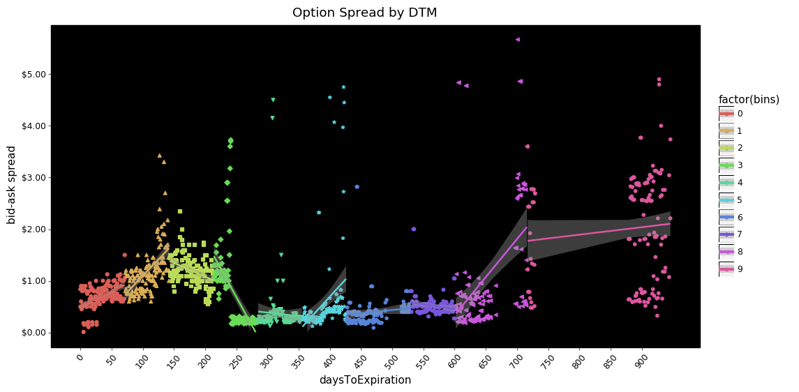
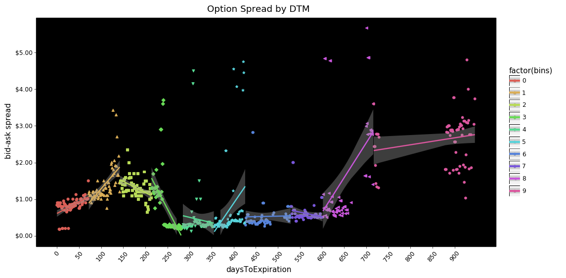
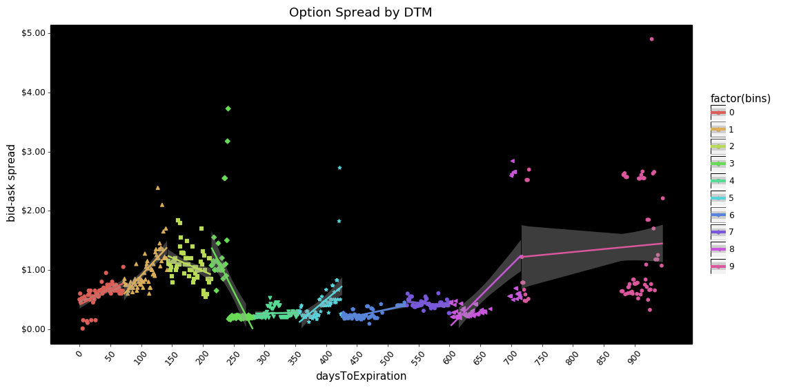
Some things are interesting. From ~250 through ~600 days in both call and put options the bid-ask spreads are compressed towards zero. There also appears to be less dispersion in put bid-ask spreads overall.
We can look at a few select ETFs.
median_sprd = data.groupby(['symbol', 'daysToExpiration', 'optionType'],
                           as_index=False)['spread'].median()

test_syms = ['SPY', 'DIA', 'QQQ', 'TLT', 'GLD', 'USO', 'SLV', 'XLF']
sel_med_sprd = median_sprd.query('symbol in @test_syms').dropna(subset=['spread'])
# to plot symbols have to cast to type str
sel_med_sprd.symbol = sel_med_sprd.symbol.astype(str)
p(sel_med_sprd.head())
p(sel_med_sprd.info())
A convenience plotting function for boxplots.
def plot_boxplot(df, x, y, optionType='Call'):
    """given df plot boxplot

    # Params
        df: pd.DataFrame()
        x: str(), column
        y: str(), column
        optionType: str()
    # Returns
        g: plotnine figure
    """
    df = df.query('optionType == @optionType')
    g = (pn.ggplot(df, pn.aes(x, y, color=f'factor({x})'))
         + pn.geom_boxplot()
         + pn.theme_linedraw()
         + pn.theme(figure_size=(12,6), panel_background=pn.element_rect(fill='black'))
         + pn.ylab('bid-ask spread')
         + pn.ggtitle(f'Selected Symbol {optionType} Option Spreads'))
    return g
g = plot_boxplot(sel_med_sprd, 'symbol', 'spread')
g.save(filename='call-option bid-ask spreads - boxplot.pdf')
g.draw();
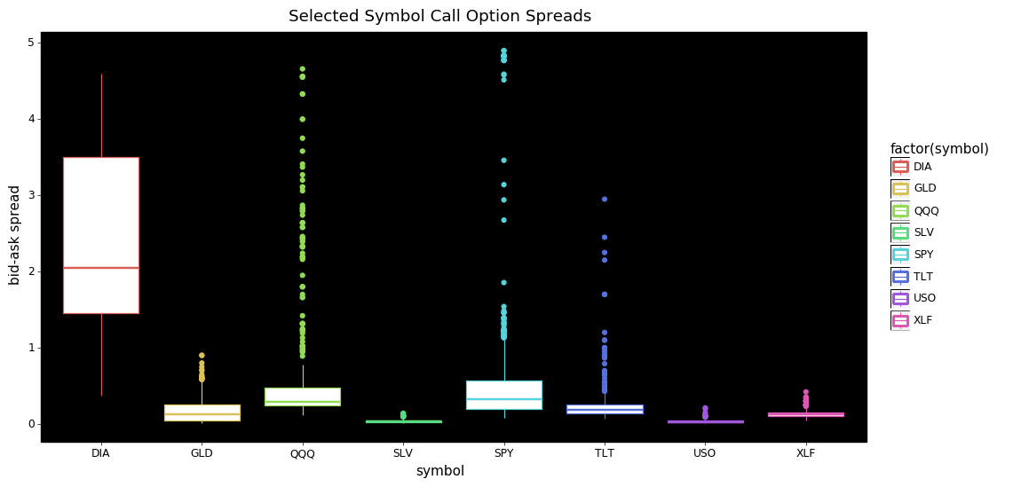
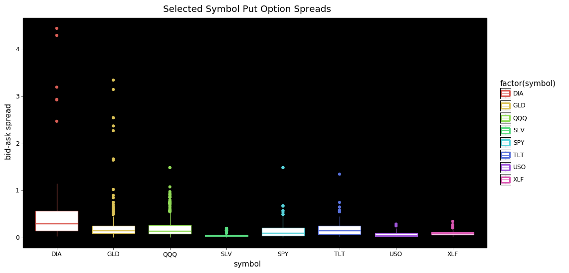
Looking at these plots we see further evidence of bid-ask spreads showing less dispersion across puts vs calls. Also it's surprising to see DIA options having such a wide range of values compared to SPY and QQQ; this is especially true for the call options.
How do bid-ask spreads Vary with volume?
grp_cols = ['symbol', 'daysToExpiration', 'optionType']
agg_cols = ['spread', 'openInterest', 'volume', 'volatility', 'intrinsic_value']
median_sprd = data.groupby(grp_cols, as_index=False)[agg_cols].median()

test_syms = ['SPY', 'DIA', 'QQQ', 'TLT', 'GLD', 'USO', 'SLV', 'XLF']
sel_med_sprd = (median_sprd.query('symbol in @test_syms')
                .dropna(subset=['spread', 'openInterest']))

# to plot symbols have to cast to type str
sel_med_sprd.symbol = sel_med_sprd.symbol.astype(str)
p(sel_med_sprd.head())
p(sel_med_sprd.info())
A convenience function for plotting...
def plot_log_points(df, x, y, color='factor(symbol)', size='openInterest'):
    g = (pn.ggplot(df, pn.aes(x, y, color=color))
         + pn.geom_point(pn.aes(size=size))
         + pn.scale_x_log10(breaks=[0,0.5,1,10,100,250,500,750,1_000])
         + pn.theme_linedraw()
         + pn.theme(figure_size=(12,6), panel_background=pn.element_rect(fill='black'),
                    axis_text_x=pn.element_text(rotation=50))
         + pn.scale_y_continuous(breaks=range(0, int(df.spread.max()+2)),
                                 labels=mzf.currency_format(), limits=(0, df.spread.max()))
         + pn.ylab('bid-ask spread'))
    return g
df = sel_med_sprd.copy()

# example with both call and puts
g = plot_log_points(df, x='volume', y='spread')
g.save(filename='call-put option bid-ask spreads - volume scatter plot.png')
g.draw();
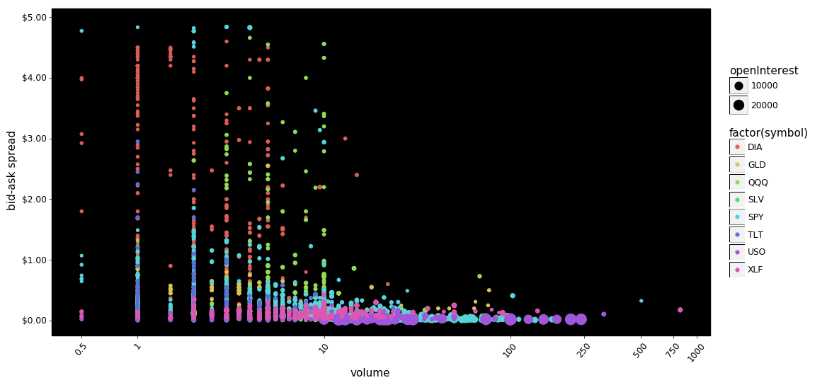
Again we see put bid-ask spreads squeezed towards zero even as volume increases. We also see SPY and USO with small spreads as both volume and open interest increases. This suggests there are symbols/contracts with higher relative trading capacity.
how do bid-ask spreads vary with volatility?
# example with both call and puts
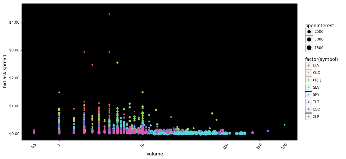
g = plot_log_points(df, 'volatility', 'spread')
g.save(filename='call-put option bid-ask spreads - volatility scatter plot.png')
g.draw();
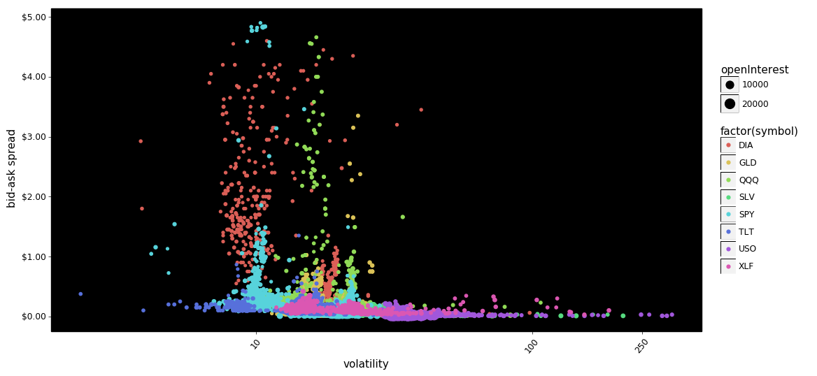
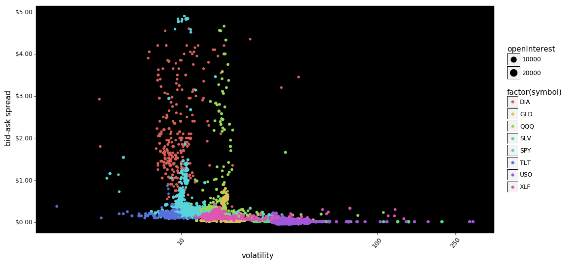
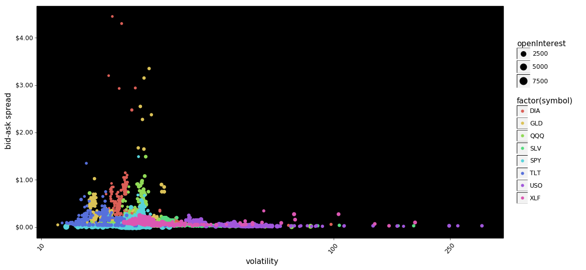
Some notes. DIA again appears to have the highest dispersion in bid-ask spreads for both calls and puts. GLD is also notable. It is also somewhat surprising that for these selected ETFs increased volatility doesn't appear with increased bid-ask spreads.
Summary Conclusions
- Put options have less overall dispersion in bid-ask spreads than calls relative to days to expiration, volume, and volatility.
- Bid-ask spreads have a major compression range between ~250 to ~600 days to maturity that appear smaller than all other buckets.
- Bid-ask spreads show greater dispersion at lower levels of implied volatility.
- DIA in particular shows the greatest variability in bid-ask spreads of the selected ETFs.
- SPY and USO show high capacity as bid-ask spreads remain near zero even at elevated volume and open interest levels.
