

Can We Use Mixture Models to Predict Market Bottoms?
/Post Outline
- Recap
- Hypothesis
- Strategy
- Conclusion
- Caveats and Areas of Exploration
- References
Recap
In Part 1 we learned about Hidden Markov Models and their application using a toy example involving a lazy pet dog. In Part 2 we learned about the expectation-maximization algorithm, K-Means, and how Mixture Models improve on K-Means weaknesses. If you still have some questions or fuzzy understanding about these topics, I would recommend reviewing the prior posts. In those posts I also provide links to resources that really helped my understanding.
Hypothesis
Given what we know about Mixture Models and their ability to characterize general distributions, can we use it to model a return series, such that we can identify outlier returns that are likely to mean revert?
Strategy
This strategy attempts to predict an asset's return distribution. Actual returns that fall outside the predicted confidence intervals are considered outliers and likely to revert to the mean.
We first fit a Gaussian Mixture Model to the historical daily return series. We use the model's estimate of the hidden state's mean and variance as parameters to a random sampling from the JohnsonSU distribution. We then calculate confidence intervals from the sampled distribution.
From there we evaluate model accuracy and the n days cumulative returns after each outlier event. We compute some summary statistics and try to answer the hypothesis.
Why the johnson SU distribution?
Searching the net I found a useful bit of code from this site. Instead of assuming our asset return distribution is normal, we can use Python and Scipy.stats to find the brute force answer. We can cycle through each continuous distribution and run a goodness-of-fit procedure called the KS-test. The KS-test is a non-parametric method which examines the distance between a known cumulative distribution function and the CDF of the your sample data. The KS-test outputs the probability that your sample data comes from the benchmark distribution.
# code sample from:
#   http://www.aizac.info/simple-check-of-a-sample-against-80-distributions/

cdfs = [
    "norm",            #Normal (Gaussian)
    "alpha",           #Alpha
    "anglit",          #Anglit
    "arcsine",         #Arcsine
    "beta",            #Beta
    "betaprime",       #Beta Prime
    "bradford",        #Bradford
    "burr",            #Burr
    "cauchy",          #Cauchy
    "chi",             #Chi
    "chi2",            #Chi-squared
    "cosine",          #Cosine
    "dgamma",          #Double Gamma
    "dweibull",        #Double Weibull
    "erlang",          #Erlang
    "expon",           #Exponential
    "exponweib",       #Exponentiated Weibull
    "exponpow",        #Exponential Power
    "fatiguelife",     #Fatigue Life (Birnbaum-Sanders)
    "foldcauchy",      #Folded Cauchy
    "f",               #F (Snecdor F)
    "fisk",            #Fisk
    "foldnorm",        #Folded Normal
    "frechet_r",       #Frechet Right Sided, Extreme Value Type II
    "frechet_l",       #Frechet Left Sided, Weibull_max
    "gamma",           #Gamma
    "gausshyper",      #Gauss Hypergeometric
    "genexpon",        #Generalized Exponential
    "genextreme",      #Generalized Extreme Value
    "gengamma",        #Generalized gamma
    "genlogistic",     #Generalized Logistic
    "genpareto",       #Generalized Pareto
    "genhalflogistic", #Generalized Half Logistic
    "gilbrat",         #Gilbrat
    "gompertz",        #Gompertz (Truncated Gumbel)
    "gumbel_l",        #Left Sided Gumbel, etc.
    "gumbel_r",        #Right Sided Gumbel
    "halfcauchy",      #Half Cauchy
    "halflogistic",    #Half Logistic
    "halfnorm",        #Half Normal
    "hypsecant",       #Hyperbolic Secant
    "invgamma",        #Inverse Gamma
    "invnorm",         #Inverse Normal
    "invweibull",      #Inverse Weibull
    "johnsonsb",       #Johnson SB
    "johnsonsu",       #Johnson SU
    "laplace",         #Laplace
    "logistic",        #Logistic
    "loggamma",        #Log-Gamma
    "loglaplace",      #Log-Laplace (Log Double Exponential)
    "lognorm",         #Log-Normal
    "lomax",           #Lomax (Pareto of the second kind)
    "maxwell",         #Maxwell
    "mielke",          #Mielke's Beta-Kappa
    "nakagami",        #Nakagami
    "ncx2",            #Non-central chi-squared
#    "ncf",             #Non-central F
    "nct",             #Non-central Student's T
    "norm"           # Normal
    "pareto",          #Pareto
    "powerlaw",        #Power-function
    "powerlognorm",    #Power log normal
    "powernorm",       #Power normal
    "rdist",           #R distribution
    "reciprocal",      #Reciprocal
    "rayleigh",        #Rayleigh
    "rice",            #Rice
    "recipinvgauss",   #Reciprocal Inverse Gaussian
    "semicircular",    #Semicircular
    "t",               #Student's T
    "triang",          #Triangular
    "truncexpon",      #Truncated Exponential
    "truncnorm",       #Truncated Normal
    "tukeylambda",     #Tukey-Lambda
    "uniform",         #Uniform
    "vonmises",        #Von-Mises (Circular)
    "wald",            #Wald
    "weibull_min",     #Minimum Weibull (see Frechet)
    "weibull_max",     #Maximum Weibull (see Frechet)
    "wrapcauchy",      #Wrapped Cauchy
    "ksone",           #Kolmogorov-Smirnov one-sided (no stats)
    "kstwobign"]       #Kolmogorov-Smirnov two-sided test for Large N

sample = data['lret'].values
for cdf in cdfs:
    try:
        #fit our data set against every probability distribution
        parameters = eval("scs."+cdf+".fit(sample)");

        #Applying the Kolmogorov-Smirnof one sided test
        D, p = scs.kstest(sample, cdf, args=parameters);

        #pretty-print the results
        D = round(D, 5)
        p = round(p, 5)

        #pretty-print the results
        print (cdf.ljust(16) + ("p: "+str(p)).ljust(25)+"D: "+str(D));
    except: continue
After running this code you should see output similar to the below code. For simplicity sake, just remember the higher the p-value, the more confident the ks-test is that our data came from the given distribution.
I had never heard of the Johnson SU distribution before this code. I had to research it, and I found that the Johnson SU was developed to in order to apply the established methods and theory of the normal distribution to non-normal data sets. What gives it this flexibility is the two shape parameters, gamma and delta, or a, b in Scipy. For more information I recommend this Wolfram reference link and this Scipy.stats link.
After selecting the distribution we can code up the experiment.
# import packages
# code was done in Jupyter Notebook

%load_ext watermark
%watermark
import pandas as pd
import pandas_datareader.data as web
import numpy as np
import sklearn.mixture as mix
import scipy.stats as scs

import matplotlib as mpl
import matplotlib.pyplot as plt
from matplotlib.dates import YearLocator, MonthLocator
%matplotlib inline

import seaborn as sns
import missingno as msno
from tqdm import tqdm

import warnings
warnings.filterwarnings("ignore")

sns.set(font_scale=1.25)
style_kwds = {'xtick.major.size': 3, 'ytick.major.size': 3,
              'font.family':u'courier prime code', 'legend.frameon': True}
sns.set_style('white', style_kwds)

p=print
p()
%watermark -p pandas,pandas_datareader,numpy,scipy,sklearn,matplotlib,seaborn
Now let's get some data.
# get fed data

f1 = 'TEDRATE' # ted spread
f2 = 'T10Y2Y' # constant maturity ten yer - 2 year
f3 = 'T10Y3M' # constant maturity 10yr - 3m

start = pd.to_datetime('2002-01-01')
end = pd.to_datetime('2017-01-01')

mkt = 'SPY'
MKT = (web.DataReader([mkt], 'yahoo', start, end)['Adj Close']
       .rename(columns={mkt:mkt})
       .assign(lret=lambda x: np.log(x[mkt]/x[mkt].shift(1)))
       .dropna())

data = (web.DataReader([f1, f2, f3], 'fred', start, end)
        .join(MKT, how='inner')
        .dropna())

p(data.head())

# gives us a quick visual inspection of the data
msno.matrix(data)
Now we create our convenience functions. The first is the run_model() function which takes the data, feature columns, and Sklearn mixture parameters to produce a fitted model object and the predicted hidden states. Note that you can use a Bayesian Gaussian mixture if you so choose. The difference between the two models is that the Bayesian mixture model will try to derive the correct number of mixture components up to a chosen maximum. For more information on the Bayesian mixture model I recommend consulting the Sklearn docs.
def _run_model(df, ft_cols, k, max_iter, init, bgm=None, **kwargs):
    """Function to run mixture model

    Params:
        df : pd.DataFrame()
        ft_cols : list of str()
        k : int(), n_components
        max_iter : int()
        init : str() {random, kmeans}

    Returns:
        model : sklearn model object
        hidden_states : array-like, hidden states
    """
    X = df[ft_cols].values

    if bgm:
        model = mix.BayesianGaussianMixture(n_components=k,
                                            max_iter=max_iter,
                                            init_params=init,
                                            **kwargs,
                                           ).fit(X)
    else:
        model = mix.GaussianMixture(n_components=k,
                                    max_iter=max_iter,
                                    init_params=init,
                                    **kwargs,
                                   ).fit(X)

    hidden_states = model.predict(X)
    return model, hidden_states
The next function takes the model object and predicted hidden states and returns the estimated mean and variance of the last state.
def _get_state_est(model, hidden_states):
    """Function to return estimated state mean and state variance

    Params:
        model : sklearn model object
        hidden_states : {array-like}
    Returns:
        mr_i : model mean return of last estimated state
        mvar_i : model variance of last estimated state
    """
    # get last state
    last_state = hidden_states[-1]
    # last value is mean return for ith state
    mr_i = model.means_[last_state][-1]
    mvar_i = np.diag(model.covariances_[last_state])[-1]
    return mr_i, mvar_i
Now we take the estimated state mean and variance of the last predicted state and feed it into the _get_ci() function. This function takes the alpha and shape parameters, estimated mean and variance and randomly samples from the JohnsonSU distribution. From this distribution we derive confidence intervals.
def _get_ci(mr_i, mvar_i, alpha, a, b, nSamples):
    """Function to sample confidence intervals from the JohnsonSU distribution

    Params:
        mr_i : float()
        mvar_i : float()
        alpha : float()
        a : float()
        b : float()
        nsamples : int()
    Returns:
        ci : tuple(float(), float()), (low_ci, high_ci)
    """
    np.random.RandomState(0)
    rvs_ = scs.johnsonsu.rvs(a, b, loc=mr_i, scale=mvar_i, size=nSamples)
    ci = scs.johnsonsu.interval(alpha=alpha, a=a, b=b,  loc=np.mean(rvs_), scale=np.std(rvs_))
    return ci
The final function visualizes our model predictions, by highlighting target returns that fell inside and outside the confidence intervals, along with our predicted confidence intervals.
def plot_pred_success(df, year, a, b):
    # colorblind safe palette http://colorbrewer2.org/
    colors = sns.color_palette('RdYlBu', 4)

    fig, ax = plt.subplots(figsize=(10, 7))
    ax.scatter(df.index, df.tgt, c=[colors[1] if x==1 else colors[0] for x in df['in_rng']], alpha=0.85)
    df['high_ci'].plot(ax=ax, alpha=0.65, marker='.', color=colors[2])
    df['low_ci'].plot(ax=ax, alpha=0.65, marker='.', color=colors[3])
    ax.set_xlim(df.index[0], df.index[-1])

    nRight = df.query('in_rng==1').shape[0]
    accuracy = nRight / df.shape[0]
    ax.set_title(r'cutoff year: {} | accuracy: {:2.3%} | errors: {} | a={}, b={}'
                  .format(year, accuracy, df.shape[0] - nRight, a, b))

    in_ = mpl.lines.Line2D(range(1), range(1), color="white", marker='o', markersize=10, markerfacecolor=colors[1])
    out_ = mpl.lines.Line2D(range(1), range(1), color="white", marker='o', markersize=10, markerfacecolor=colors[0])
    hi_ci = mpl.lines.Line2D(range(1), range(1), color="white", marker='.', markersize=15, markerfacecolor=colors[2])
    lo_ci = mpl.lines.Line2D(range(1), range(1), color="white", marker='.', markersize=15, markerfacecolor=colors[3])
    leg = ax.legend([in_, out_, hi_ci, lo_ci],["in", "out", 'high_ci', 'low_ci'],
                    loc = "center left", bbox_to_anchor = (1, 0.85), numpoints = 1)
    sns.despine(offset=2)
    plt.tight_layout()
    return
Now we can run the model in a walk-forward fashion. The code uses a chosen lookback period up until the cutoff year to fit the model. From there, the code iterates refitting the model each day, outputting the predicted confidence intervals. The code is setup to run using successive cutoff years, however I will leave that to you readers to experiment with. In this demo we will break the loop after the first cutoff year.
%%time

# Model Params
# ------------
a, b = (.2, .7) # found via coarse parameter search
alpha = 0.99
max_iter = 100
k = 2
init = 'random' #'kmeans'
nSamples = 2_000
ft_cols = [f1, f2, f3, 'lret']

years = range(2009,2016)
lookback = 1 # chosen for ease of computation

# Iterate Model
# ------------
for year in years:
    cutoff = year
    train_df = data.ix[str(cutoff - lookback):str(cutoff)].dropna()
    oos = data.ix[str(cutoff+1):].dropna()
    # confirm that train_df end index is different than oos start index
    assert train_df.index[-1] != oos.index[0]

    # create pred list to hold tuple rows
    preds = []
    for t in tqdm(oos.index):
        if t == oos.index[0]:
            insample = train_df

        # run model func to return model object and hidden states using params
        model, hstates = _run_model(insample, ft_cols, k, max_iter, init, random_state=0)
        # get hidden state mean and variance
        mr_i, mvar_i = _get_state_est(model, hstates)
        # get confidence intervals from sampled distribution
        low_ci, high_ci = _get_ci(mr_i, mvar_i, alpha, a, b, nSamples)
        # append tuple row to pred list
        preds.append((t, hstates[-1], mr_i, mvar_i, low_ci, high_ci))

        # increment insample dataframe
        insample = data.ix[:t]

    cols = ['ith_state', 'ith_ret', 'ith_var', 'low_ci', 'high_ci']
    pred = (pd.DataFrame(preds, columns=['Dates']+cols)
            .set_index('Dates').assign(tgt = oos['lret']))

    # logic to see if error exceeds neg or pos CI
    pred_copy = pred.copy().reset_index()
    # Identify indices where target return falls between CI
    win = pred_copy.query("low_ci < tgt < high_ci").index
    # create list of binary variables representing in/out CI
    in_rng_list = [1 if i in win else 0 for i in pred_copy.index]
    # assign binary variables sequence to new column
    pred['in_rng'] = in_rng_list

    plot_pred_success(pred, year, a, b)
    break

After that's complete we need to set up our analytics functions to evaluate the return patterns post each event. Recall that an event is an actual return that fell outside of our predicted confidence intervals.
def post_event(df, event, step_fwd=None):
    """Function to return dictionary where key, value is integer
    index, and Pandas series consisting of returns post event

    Params:
        df : pd.DataFrame(), prediction df
        event : {array-like}, index of target returns that exceed CI high or low
        step_fwd : int(), how many days to include after event
    Returns:
        after_event : dict()
    """
    after_event = {}
    for i in range(len(event)):
        tmp_ret = df.ix[event[i]:event[i]+step_fwd, ['Dates','tgt']]
        # series of returns with date index
        after_event[i] = tmp_ret.set_index('Dates', drop=True).squeeze()
    return after_event

def plot_events_timeline(post_events, event_state):
    fig, ax = plt.subplots(figsize=(10, 7))
    ax.axhline(y=0, color='k', lw=3)
    for k in post_events.keys():
        tmp = post_events[k].copy()
        tmp.iloc[0] = 0 # set initial return to zero

        if tmp.sum() > 0: color = 'dodgerblue'
        else: color = 'red'
        ax.plot(tmp.index, tmp.cumsum(), color=color, alpha=0.5)
        ax.set_xlim(pd.to_datetime('2009-12-31'), tmp.index[-1])
        ax.set_xlabel('Dates')
        ax.set_title(f"{mkt} {event_state.upper()}", fontsize=16, fontweight='demi')
        sns.despine(offset=2)
    return

def plot_events_post(post_events, event_state):
    fig, ax = plt.subplots(figsize=(10, 7))
    ax.axhline(y=0, color='k', lw=3)
    for k in post_events.keys():
        tmp = post_events[k].copy()
        tmp.iloc[0] = 0 # set initial return to zero

        if tmp.sum() > 0: color = 'dodgerblue'
        else: color = 'red'
        tmp.cumsum().reset_index(drop=True).plot(color=color, alpha=0.5, ax=ax)
    ax.set_xlabel('Days')
    ax.set_title(f"{mkt} {event_state.upper()}", fontsize=16, fontweight='demi')
    sns.despine(offset=2)
    return

def plot_distplot(ending_values, summary):
    colors = sns.color_palette('RdYlBu', 4)
    fig, ax = plt.subplots(figsize=(10, 7))
    sns.distplot(pd.DataFrame(ending_values), bins=15, color=colors[0],
                 kde_kws={"color":colors[3]}, hist_kws={"color":colors[3], "alpha":0.35}, ax=ax)
    ax.axvline(x=float(summary['mean'][0]), label='mean', color='dodgerblue', lw=3, ls='-.')
    ax.axvline(x=float(summary['median'][0]), label='median', color='red', lw=3, ls=':')
    ax.axvline(x=0, color='black', lw=1, ls='-')
    ax.legend(loc='best')
    sns.despine(offset=2)
    ax.set_title(f"{mkt} {event_state.upper()}", fontsize=16, fontweight='demi')
    return

def get_end_vals(post_events):
    """Function to sum and agg each post events' returns"""
    end_vals = []
    for k in post_events.keys():
        tmp = post_events[k].copy()
        tmp.iloc[0] = 0 # set initial return to zero
        end_vals.append(tmp.sum())
    return end_vals

def create_summary(end_vals):
    gt0 = [x for x in end_vals if x>0]
    lt0 = [x for x in end_vals if x<0]
    assert len(gt0) > 1
    assert len(lt0) > 1
    summary = (pd.DataFrame(index=['value'])
               .assign(mean = f'{np.mean(end_vals):.4f}')
               .assign(median = f'{np.median(end_vals):.4f}')
               .assign(max_ = f'{np.max(end_vals):.4f}')
               .assign(min_ = f'{np.min(end_vals):.4f}')
               .assign(gt0_cnt = f'{len(gt0):d}')
               .assign(lt0_cnt = f'{len(lt0):d}')
               .assign(sum_gt0 = f'{sum(gt0):.4f}')
               .assign(sum_lt0 = f'{sum(lt0):.4f}')
               .assign(sum_ratio = f'{sum(gt0) / abs(sum(lt0)):.4f}')
               .assign(gt_pct = f'{len(gt0) / (len(gt0) + len(lt0)):.4f}')
               .assign(lt_pct = f'{len(lt0) / (len(gt0) + len(lt0)):.4f}')
               )
    return summary
Now we can run the following code to extract the events, output the plots and view the summary.
df = pred.copy().reset_index()
too_high = df.query("tgt > high_ci").index
too_low = df.query("tgt < low_ci").index

step_fwd=5 # how many days to look forward
event_states = ['too_high', 'too_low']
for event in event_states:

    after_event = post_event(df, eval(event), step_fwd=step_fwd)
    ev = get_end_vals(after_event)
    smry = create_summary(ev)
    p()
    p('*'*25)
    p(mkt, event.upper())
    p(smry.T)

    plot_events_timeline(after_event, event)
    plot_events_post(after_event, event)
    plot_distplot(ev, smry, event)


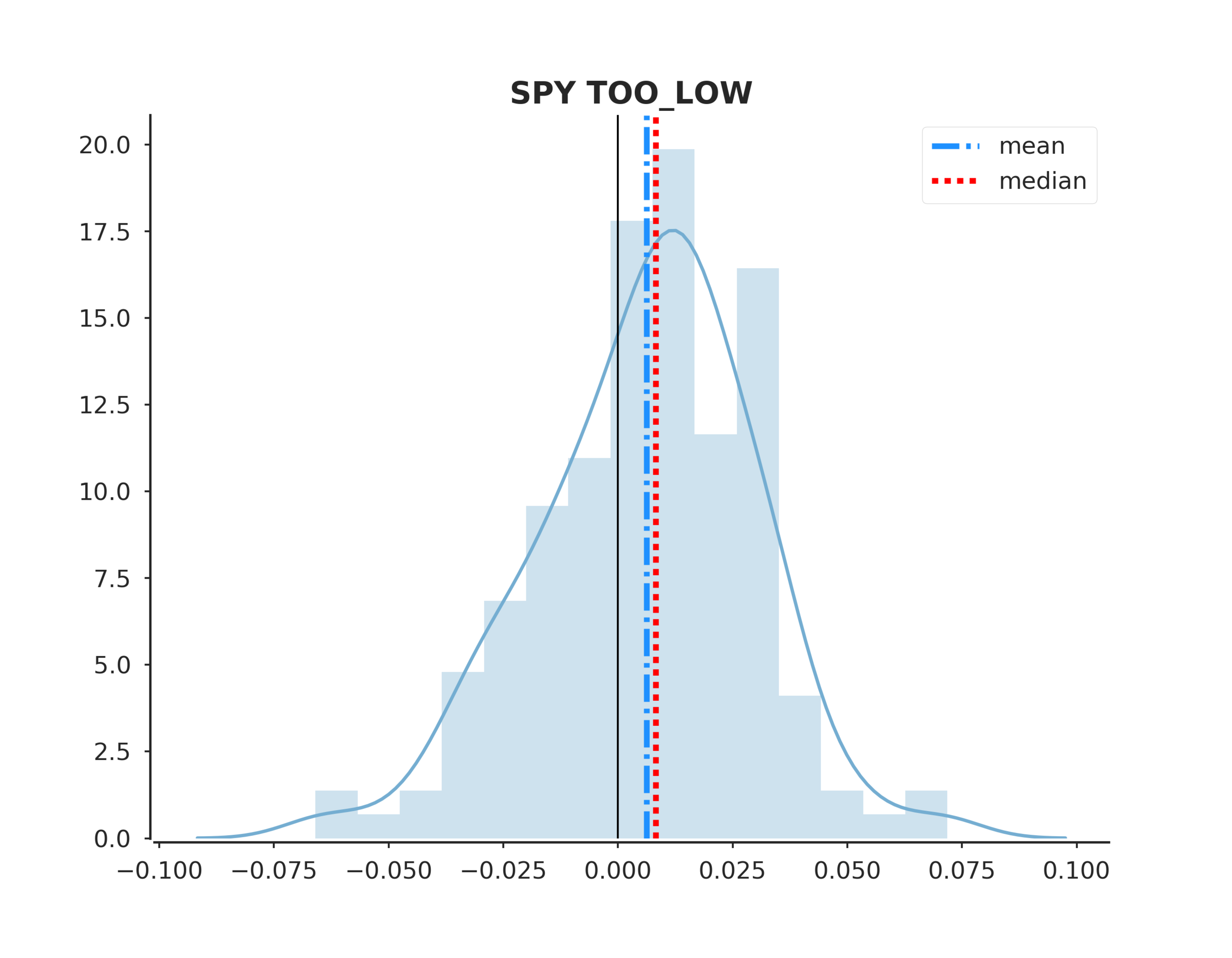


Conclusions
To answer the original hypothesis about finding market bottoms, we can examine the returns after a too low event. Looking at the summary we can see that the mean and median return are +62 and +82 bps respectively. Looking at the sum_ratio we can see that that the sum of all positive return events is almost 2x the sum of all negative returns. We can also see that, given a too low event, after 5 days SPY had positive returns 65% of the time!
These are positive indicators that we may be able to predict market bottoms. However, I would emphasize more testing is needed.
Caveats and Areas of Exploration
- We don't consider market frictions such as commissions or slippage
- The daily prices may or may not represent actual traded values.
- I used a coarse search to find the JohnsonSU shape parameters, a and b. These may or may not be the best values. Just note that we can use these parameters to arbitrarily adjust the confidence intervals to be more or less conservative. I leave this for the reader to explore.
- In many cases both too high, and too low events result in majority positive returns, this could be an indication of the overall bullishness of the sample period that may or may not affect model results in the future.
- I chose k=2 components for computational simplicity, but there may be better values.
- I chose the lookback period for computational simplicity, but there may be better values.
- Varying the step_fwd parameter may hurt or hinder the strategy.
- What makes this approach particularly interesting, is that we don't want anything close to 100% accuracy from our predicted confidence intervals, otherwise we won't have enough "trades". This adds a level of artistry/complexity because the parameter values we choose should create predictable mean reversion opportunities, but the model accuracy is not a good indicator of this. Testing the strategy with other assets shows "profitability" in some cases where the model accuracy is sub 60%.
Please contact me if you find any errors.
