

A Dead Simple 2-Asset Portfolio that Crushes the S&P500 (Part 2)
/In Part 1, and Part 1.5 I introduced a simple 2-asset portfolio that substantially outperformed the SPY ETF since 2009. In Part 1 I examined the performance of an "inverse risk-parity" approach where the ETF with the largest volatility contribution to the portfolio was weighted more heavily. In Part 1.5 I examined the performance of the actual "risk-parity" approach, where the ETF with the smallest volatility contribution is weighted more heavily. In this post I will examine some of the conceptual foundations underlying the strategy.
Leveraged ETFs and Beta Slippage
Suppose you are considering a position in a leveraged ETF (LETF). You aren't familiar with the specific quirks of LETF performance but decide to take the plunge anyways. You purchase $1 each of the unlevered ETF, the 2x levered ETF, and the 3x levered ETF in an attempt to learn by doing. Over the next 2 days the unlevered ETF increases +11.2% and then declines -10%. The value of each initial $1 portfolio is calculated below:
# first return path
rs = pd.Series([.112, -.10])
rs_2x = rs * 2
rs_3x = rs * 3

rs_comp = np.cumprod(1+rs)
rs_2x_comp = np.cumprod(1+rs_2x)
rs_3x_comp = np.cumprod(1+rs_3x)

print("return series volatility: {:3.2%}".format(rs.std()))
print("approximate value of unlevered portfolio: {} | beta slippage: {}"
      .format(rs_comp.values, rs_comp.iloc[-1] - rs_comp.iloc[-1]))
print("approximate value of 2x leverage portfolio: {} | beta slippage: {:.5}"
      .format(rs_2x_comp.values, rs_2x_comp.iloc[-1] - rs_comp.iloc[-1]))
print("approximate value of 3x leverage portfolio: {} | beta slippage: {:.5}"
      .format(rs_3x_comp.values, rs_3x_comp.iloc[-1] - rs_comp.iloc[-1]))
You see the results and clearly something must be wrong right? After 2 days the unlevered portfolio is essentially unchanged in value while the 2x and 3x have lost ~2% and ~6.6% respectively!
You liquidate all 3 portfolios and decide to try again with the same unlevered ETF. You repeat the process and allocate $1 each to the unlevered ETF, the 2x levered ETF, and the 3x levered ETF. Over the next 2 days the unlevered ETF increases +20% and then declines -16.67%. The value of each initial $1 portfolio is calculated below.
# second return path
rs = pd.Series([.20, -.1667])
rs_2x = rs * 2
rs_3x = rs * 3

rs_comp = np.cumprod(1+rs)
rs_2x_comp = np.cumprod(1+rs_2x)
rs_3x_comp = np.cumprod(1+rs_3x)

print("return series volatility: {:3.2%}".format(rs.std()))
print("approximate value of unlevered portfolio: {} | beta slippage: {}"
      .format(rs_comp.values, rs_comp.iloc[-1] - rs_comp.iloc[-1]))
print("approximate value of 2x leverage portfolio: {} | beta slippage: {:.5}"
      .format(rs_2x_comp.values, rs_2x_comp.iloc[-1] - rs_comp.iloc[-1]))
print("approximate value of 3x leverage portfolio: {} | beta slippage: {:.5}"
      .format(rs_3x_comp.values, rs_3x_comp.iloc[-1] - rs_comp.iloc[-1]))
Now you're really pissed because this time the slippage is worse. After 2 days the unlevered ETF is again nearly unchanged and yet the 2x and 3x LETFs have lost ~6.6% and ~20% in value! What is happening?!
This is the natural result of managing and rebalancing a leveraged portfolio. To see why let's examine what happens after day 1 for the 3x leverage portfolio for second return path. First a simple formula for reference:
Leverage Ratio = Assets / Equity = Assets / (Assets - Borrowings)
At time 0 you owned $3 of assets for your $1 equity investment for a leverage ratio of 3x ((3 * $1)/$1 = 3x). After day 1, the unlevered ETF increased +20% and your 3x leveraged ETF investment increased +60%. So far so good, but wait, what has happened to the leverage ratio!?
(3 * 1.6) /1.6 = 2.25x
Uh-oh the 3x ETF has lost 25% of its leverage. The fund must now buy more stocks to rebalance the portfolio to the mandated leverage ratio! Rebalancing a leveraged portfolio requires the levered ETF provider to trade in the same direction of the previous move. In other words the fund must buy high and sell low in order to maintain constant leverage!
Also note that the beta slippage is a function of volatility. In the two hypothetical examples the first return path had an estimated volatility of ~15% while the second return path was an estimated ~26%. Note the following relationships:
voldelta = 25.93 / 14.99 - 1
x2 = -0.06672/-0.0216 - 1
x3 = -0.20012/-0.0656 - 1
print("change in volatility between return paths 1 and 2: {:3.2%}\n".format(voldelta))
print("change in beta slippage between return paths 1 and 2:\n2x leverage: {:3.2%}\n3x leverage: {:3.2%}"
      .format(x2, x3))
Volatility increased ~73% and yet the beta slippage increased ~209% and 205% between the 2x and 3x levered ETFs respectively. We can see that the relationship between changes in return volatility and changes in beta slippage is positive and nonlinear. Another name that describes a nonlinear change in output for a change in input is convexity.
Beta Slippage depends on a specific return sequence and is positively related to the volatility of returns. As the volatility increases so does the beta slippage.
Using a toy example to help illustrate this concept let's create 10,000 samples of simulated two day (un)levered returns. From there we calculate and sort the samples by volatility and observe the relationship between volatility and beta slippage. First some convenience functions (Notice below I calculate the beta slippage as the unlevered portfolio value on day 2 minus the levered portfolio value on day 2):
def volatility(inc_returns, dec_returns):
    """create dataframe and calculate return volatility and change in volatility"""
    df = pd.DataFrame({'day_1':inc_returns, 'day_2':dec_returns}, index=range(len(inc_returns)))
    df['volatility'] = df[['day_1', 'day_2']].std(axis=1)
    df = df.sort_values('volatility')
    df['voldelta'] = df['volatility'] / df['volatility'].shift(1) - 1
    return df

def levered_returns(df):
    """calculate levered and unlevered returns"""
    df['unlevered_portV_day2'] = np.cumproduct(1 + df[['day_1', 'day_2']], axis=1).iloc[:,-1]
    df['2x_day1_returns'] = df['day_1'] * 2
    df['3x_day1_returns'] = df['day_1'] * 3
    df['2x_day2_returns'] = df['day_2'] * 2
    df['3x_day2_returns'] = df['day_2'] * 3
    return df


def beta_slippage(df):
    """calculate beta slippage"""

    # cuml 2x, 3x leverage returns
    df['2x_portV_day2'] = np.cumproduct(1 + df[['2x_day1_returns', '2x_day2_returns']], axis=1).iloc[:,-1]
    df['3x_portV_day2'] = np.cumproduct(1 + df[['3x_day1_returns', '3x_day2_returns']], axis=1).iloc[:,-1]

    # calc beta slippage
    df['2x_beta_slippage'] = df['unlevered_portV_day2'] - df['2x_portV_day2']
    df['3x_beta_slippage'] = df['unlevered_portV_day2'] - df['3x_portV_day2']

    df = df.dropna().reset_index(drop=True)
    reidx_cols = ['day_1', 'day_2', '2x_day1_returns', '2x_day2_returns',
                  '3x_day1_returns', '3x_day2_returns',
                  'unlevered_portV_day2', '2x_portV_day2', '3x_portV_day2',
                  'volatility', 'voldelta', '2x_beta_slippage', '3x_beta_slippage'
                 ]
    df = df.reindex(columns = reidx_cols)
    return df
Next create the dataset and dataframe:
seed = np.random.seed(10)
inc_returns = pd.Series(n + np.random.uniform(.02,.1) for n in np.linspace(.01, .25, 10000))
dec_returns = pd.Series(n + np.random.uniform(.02,.1) for n in np.linspace(.01, .2, 10000)) * -1
tf = volatility(inc_returns, dec_returns)
tf = levered_returns(tf)
tff = beta_slippage(tf)
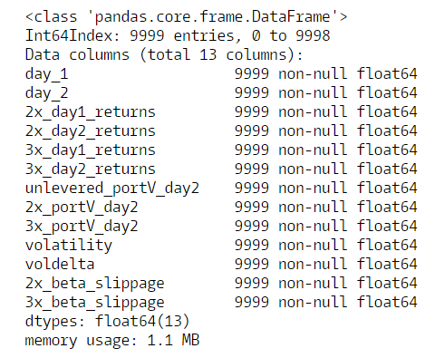
print(tff.info())
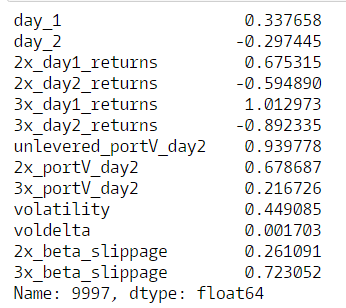
max_loc_3x = tff['3x_beta_slippage'].argmax()
print(tff.loc[max_loc_3x])
Now we can look at a visual representation of the relationship between beta slippage volatility.

As expected as volatility increases beta slippage increases. We can also see that leverage exacerbates this effect as the 3x slippage increases at a faster rate than the 2x. We can also see the nonlinear nature of the relationship. Slippage can be positive or negative at smaller levels of volatility. The blur effect exhibited by the data points indicates that beta slippage is heavily dependent on the actual return path at each level of volatility.
How correlated is beta slippage with volatility?


Simple linear regression shows correlations are greater than 80%. Finally to highlight the nonlinearity of this relationship I plot the beta slippage rate of change vs the volatility rate of change.
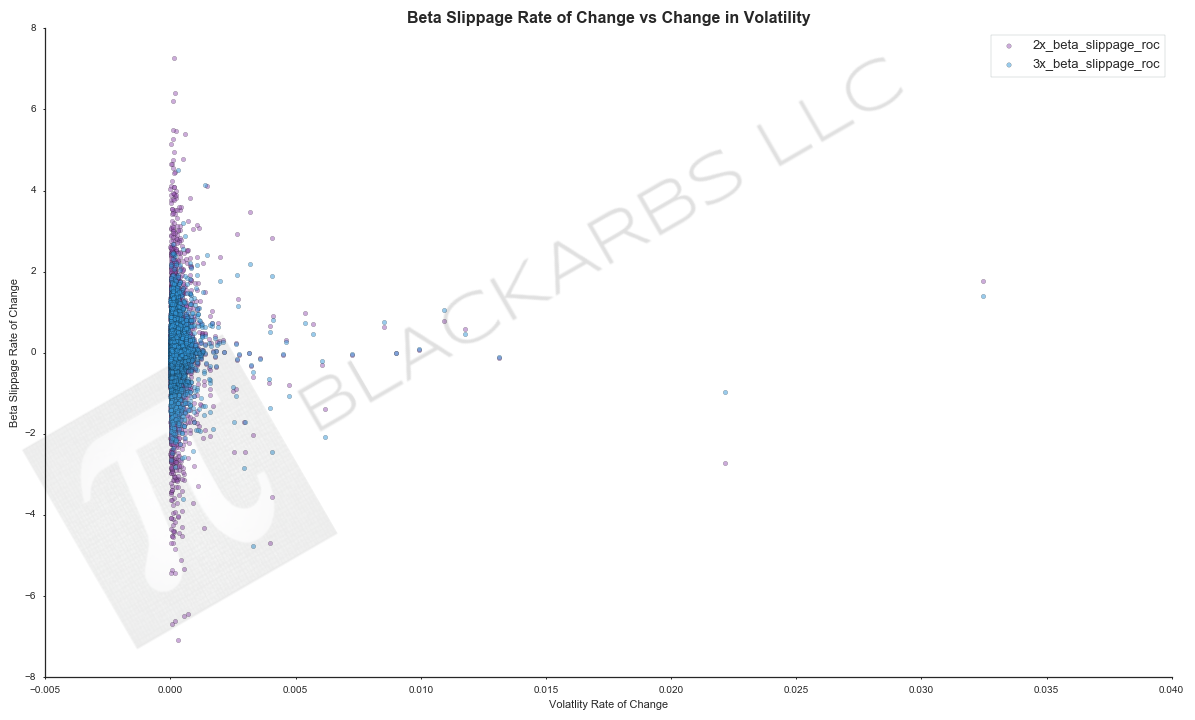
Changes in beta slippage are highly sensitive to changes in volatility.
See the upcoming Part 2.5 where I examine the relationship between the underlying strategy ETFs, SPY and TLT.
