

A Dead Simple 2-Asset Portfolio that Crushes the S&P500 (Part 3)
/Recap
This is an update to the original blog series that explored a simple strategy of being long UPRO and TMF in equal weight, inverse volatility and inverse-inverse volatility. This strategy crushed the cumulative and risk-adjusted returns of the benchmark SPY etf. However through our research we determined that this strategy is heavily dependent on the correlation between the two assets. This strategy works best when correlations are positive and prices are trending positively, however, theoretically it is most stable when correlations are negative. Previously we determined the strategy is most exposed when correlations are positive or rising and prices are declining. The problem is that we don’t know ex-ante if, during periods of increasing correlations, prices will trend up or down, which exposes our capital to large risks. In the past I eluded to a potential workable solution to this issue. In this blog post and associated materials we will explore some potential solutions to this problem.
Outline
Introduction
Setup
Correlations
Strategy Goals
Prototype Strategies
Results
Conclusions
Future Work
References
Introduction
In the first portion of this experiment, we will rehash the previous analysis of conditional returns based on correlation, this time using a higher quality dataset resampled from a 1 minute resolution. We will also explore conditional returns based on the information theoretic measure of Mutual Information. The benefit of mutual information is that it is designed to detect linear and non-linear relationships. The values are between 0 and 1 with a relatively simplified interpretation that 0 means no relationship (or no shared information between random variables), while a 1 means a perfect relationship (or total information shared between random variables). Note that this is a more generalized metric than correlation, which only captures linear dependency.
From there we will setup the benchmark, determine our strategy goals, and potential improvements. We will evaluate the prototype strategies using Pyfolio and ffn modules to get a quick understanding if any of our adjustments have improved the strategy. If these updates show promise then we will move forward with a more comprehensive implementation within the Quantconnect platform.
Setup
This analysis was run in a Jupyter notebook. What follows is are my imports. Please note that some functions and tools are stored within a local project package. If the functions they import are required I will reproduce them here or attach a python file that contains the code for the functions. Also note not all the imports are required. For example, I import a package called modin.pandas which is made to replicate the original pandas yet use multiprocessing in the backend. For those who prefer to use the regular version of pandas that will work too. Also I use the package gcmi for the mutual information calculations. See the link for instructions on how to install and use the package.
%load_ext watermark
%watermark

%load_ext autoreload
%autoreload 2

# import standard libs
import warnings
warnings.filterwarnings("ignore")
from IPython.display import display
from pathlib import Path

# import python scientific stack
import modin.pandas as pd
#import pandas as pd
pd.set_option('display.max_rows', 100)
import numpy as np
import scipy.stats as stats
import statsmodels.api as sm
import numba as nb
import pyfolio as pf
import ffn

# import visual tools
from PIL import Image, ImageOps
import matplotlib as mpl
import matplotlib.pyplot as plt
import matplotlib.gridspec as gridspec
%matplotlib inline
import seaborn as sns

# import util libs
from tqdm import tqdm, tqdm_notebook
import missingno as msno
from algo_dev.CONSTANTS import REPO_NAME
from algo_dev.tools.utils import *
import algo_dev.tools.gcmi as gcmi

print('\n',REPO_NAME)
pdir = get_relative_project_dir(REPO_NAME)
data_dir = pdir/'data'
external = data_dir/'external'
processed = data_dir/'processed'

print()
%watermark --iversion
I split these imports into 2 blocks because I also use an extension called nb_black which is an automatic code formatter which will make your code look clean and easier to interpret.
%load_ext nb_black


sns_params = {
    "xtick.major.size": 2,
    "ytick.major.size": 2,
    "font.size": 11,
    "font.weight": "medium",
    "figure.figsize": (10, 7),
    "font.family": "Ubuntu Mono",
}

sns.set_style("white", sns_params)
sns.set_context(sns_params)
savefig_kwds = dict(dpi=300, bbox_inches="tight", frameon=True, format="png")
flatui = ["#3498db", "#9b59b6", "#95a5a6", "#e74c3c", "#34495e", "#2ecc71", "#f4cae4"]
sns.set_palette(sns.color_palette(flatui, 7))


def save_image(fig, fn):
    fig.savefig(Path(viz / fn).as_posix(), **savefig_kwds)
    print(f"image saved: {fn}")
    return

Package Import versions
The data set is 1 min trade data from tradestation (no affiliation). I cannot share this data due to the terms of use but it is easy and simple to get access to a lot of data from tradestation and I don’t think they have any account minimums. One thing is their platform only works for Windows, so if you have linux you will have to use a virtual box to run it.
Get Data
def read_tradestation_data(fp):
    df = (
        pd.read_csv(fp)
        .assign(
            datetime=lambda df: pd.to_datetime(
                (df.Date + " " + df.Time), infer_datetime_format=True
            )
        )
        .set_index("datetime")
        .drop(["Date", "Time"], axis=1)
    )
    df.columns = df.columns.str.lower()
    return df

symbols = ["UPRO", "TMF"]
dfs = list()

for sym in tqdm(symbols):
    etf_dir = external / "tradestation"
    fp = etf_dir / f"{sym}.txt"
    tmp_df = read_tradestation_data(fp).assign(symbol=sym)
    dfs.append(tmp_df)

df = pd.concat(dfs, axis=0)
cprint(df)
RESAMPLE
close = (
    df.groupby("symbol")["close"]
    .resample("30Min")
    .ohlc()
    .dropna()["close"]
    .unstack(0)
    .sort_index()
    .dropna()
)
cprint(close)
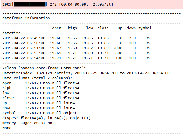
EXAMPLE OF RESAMPLED DATA.
resampled price series.
LOG RETURNS
R = np.log(close / close.shift(1)).dropna()
CORRELATIONS
rollcorr = R.rolling(int(6 * 252)).corr(pairwise=True).dropna()

def roll_avg_corr(df_corr):
    """
    compute rolling average pairwaise correlation

    see:
        https://stackoverflow.com/questions/44914845/rolling-mean-of-correlation-matrix

    :param pd.DataFrame df_corr: df with datetime as index and corr matrix for each date
    :return pd.Series: average pairwise correlations

    Example of df_corr:
        symbol                           TMF      UPRO
        datetime            symbol
        2010-04-13 09:00:00 TMF     1.000000 -0.328035
                            UPRO   -0.328035  1.000000
        2010-04-13 10:00:00 TMF     1.000000 -0.329089
                            UPRO   -0.329089  1.000000
        2010-04-13 11:00:00 TMF     1.000000 -0.331043
    """
    mask = np.triu_indices(df_corr.shape[1], k=1)
    dates = df_corr.index.get_level_values(0)
    avgs = [df_corr.loc[date].values[mask].mean() for date in dates]
    s = pd.Series(avgs, index=dates).rename("average_pairwise_correlation")
    return s


avg_corr = roll_avg_corr(rollcorr).drop_duplicates()
MUTUAL INFORMATION
def roll_gcmi(R, step=int(6 * 252)):
    roll_mi_list = list()
    for i, _ in enumerate(tqdm_notebook(R.index[step + 1 :]), start=step + 1):
        x, y = R.iloc[i - step : i, 0], R.iloc[i - step : i, 1]
        xx = x.drop_duplicates()
        yy = y.drop_duplicates()
        idx = xx.index.intersection(yy.index)
        xx = xx.loc[idx]
        yy = yy.loc[idx]
        try:
            tmp = gcmi.gcmi_cc(xx, yy)
        except:
            tmp = np.nan
        roll_mi_list.append((_, tmp))

    roll_mi = pd.DataFrame(roll_mi_list, columns=["datetime", "mi"]).set_index(
        "datetime"
    )
    return roll_mi


roll_mi = roll_gcmi(R, step=int(6 * 252))
We can see that there is a seemingly inverse relationship between the correlation and mutual information in this particular case.
returns given average correlation is decreasing
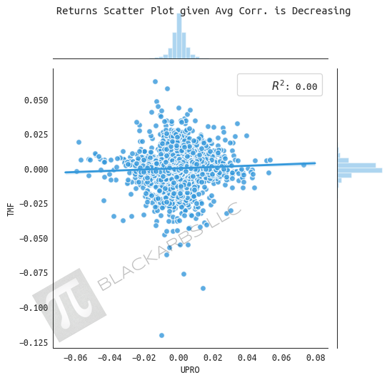

UPRO appears to have stable increasing returns when average correlation is decreasing (correlation moving towards to zero). TMF underperforms with a decreasing trend over time.
RETURNS GIVEN MUTUAL INFORMATION IS DECREASING
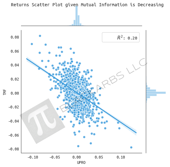

When the mutual Information of the two assets is declining it appears as if both assets and the Index trend upwards.
RETURNS GIVEN AVERAGE CORRELATION INCREASING
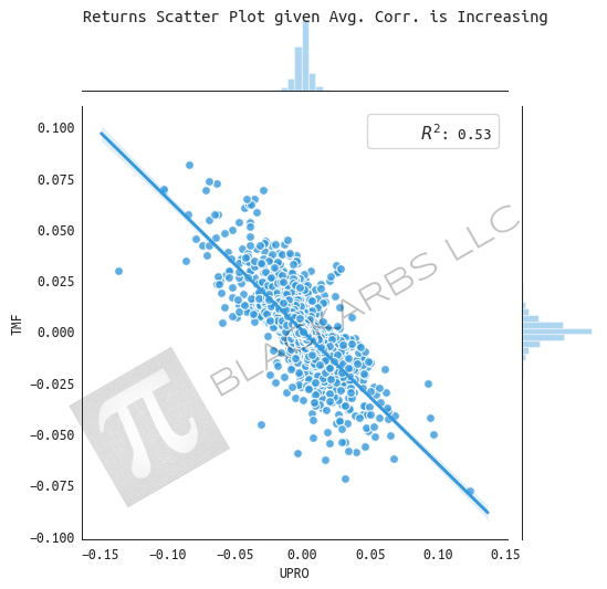

We see TMF outperform when average correlation is increasing (becoming more negative, and in rare cases, increasingly positive). Overall returns from the Index trend higher compared to the decreasing state, almost doubling the cumulative return.
RETURNS GIVEN MUTUAL INFORMATION IS INCREASING


When mutual information is increasing UPRO is very strong while TMF is mostly negative but there is 20% difference between the performance of the Index between the two states. When M.I. is decreasing, the cumulative sum is 0.99 compared to 0.82. However I don’t know if anything economically significant can be drawn from this distinction.
NOTE:
I ran this analysis on multiple resampled resolutions including 10 minute, 30 minute, 1 hour, 2 hour, 4 hour and daily. The results were mostly similar across all resolutions except for the 1 hour. For some reason, that particular resolution, all the results were inverted in terms of performance. It is a strange phenomenon but I would like readers to be aware of these peculiarities when working with resampled data.
Strategy Goals
As we will see below the original UPRO + TMF returns over 1000% over the backtest period. Even the risk-adjusted metrics are solid given the simplicity of the strategy. However, my issues with the strategy are the drawdown depth, and length of drawdowns. My personal preference is a strategy that is lower volatility, low drawdowns and shorter drawdown periods.
Thus the goals to improve the strategy are to reduce drawdowns to below 15% or less but really 10% is ideal. Preferably we can get max drawdown durations to less than 6 months, and positive returns each year for the backtest period. Ideally we can try to achieve this with minimal data-mining or optimization.
The reason for the focus on drawdown versus total returns is that realistically it will be hard to stay invested in a algorithmic strategy with a drawdown of 20% of invested equity for 10 months.
Prototype Strategies
Below we'll be evaluating some prototype strategies to see if we can improve on the `risk-adjusted` performance of the benchmark UPRO-TMF Equal weight strategy. To do this we will be using pyfolio and ffn packages to evaluate relevant metrics. Note that for some reason pyfolio is not computing the correct performance metrics even though the plot displays seem to be correct. This is also why we will use ffn for comparison.
NOTE
The following analysis does not incorporate transaction costs like commissions, slippage, or price impact. The purpose is to evaluate prototype strategies to understand which, if any, strategies are worth exploring further using more a more realistic backtest environment.
def to_price_index(df, start=1):
    return start * (np.exp(df.cumsum()))

def common_sense_ratio(returns):
    # common sense ratio
    ratio = (abs(returns.quantile(0.95)) * returns[returns > 0].sum()) / abs(
        abs(returns.quantile(0.05)) * returns[returns < 0].sum()
    )
    ratio = round(ratio, 2)
    return ratio


def plot_pf(returns):
    plots = [
        pf.plot_rolling_returns,
        pf.plot_annual_returns,
        pf.plot_monthly_returns_heatmap,
        pf.plot_monthly_returns_dist,
        pf.plot_drawdown_underwater,
    ]

    fig = plt.figure(figsize=(12, 10))
    gs = gridspec.GridSpec(3, 3, height_ratios=[1.0, 1, 1])

    for i, func in enumerate(plots):

        if i == 0:
            ax = plt.subplot(gs[0, :])
            func(returns, ax=ax)
        elif i < 4:
            ax = plt.subplot(gs[1, i - 1])
            func(returns, ax=ax)
        elif i == 4:
            ax = plt.subplot(gs[2, :])
            func(returns, ax=ax)
        else:
            continue

    plt.tight_layout()


# keep_stats = test.index[0:7].tolist() + test.index[16:].tolist()
keep_stats = [
    "start",
    "end",
    "rf",
    "total_return",
    "cagr",
    "max_drawdown",
    "calmar",
    "daily_sharpe",
    "daily_sortino",
    "daily_mean",
    "daily_vol",
    "daily_skew",
    "daily_kurt",
    "best_day",
    "worst_day",
    "monthly_sharpe",
    "monthly_sortino",
    "monthly_mean",
    "monthly_vol",
    "monthly_skew",
    "monthly_kurt",
    "best_month",
    "worst_month",
    "yearly_sharpe",
    "yearly_sortino",
    "yearly_mean",
    "yearly_vol",
    "yearly_skew",
    "yearly_kurt",
    "best_year",
    "worst_year",
    "avg_drawdown",
    "avg_drawdown_days",
    "avg_up_month",
    "avg_down_month",
    "win_year_perc",
    "twelve_month_win_perc",
]


def view_strats(strats):
    return ffn.calc_stats(strats).stats.loc[keep_stats]


strats = pd.DataFrame()
BENCHMARK
First up is the benchmark version which is equal weight UPRO and TMF.
benchmark = np.exp(R[["TMF", "UPRO"]]) - 1
benchmark = benchmark.mean(axis=1)
strats["benchmark"] = benchmark
All returns hypothetical and simulated. past performance does not necessarily predict future performance.
EQUAL RISK CONTRIBUTION
# get monthly dates
date_range = simple_R.groupby(pd.TimeGrouper("1M")).sum().index

# iterate over the date range computing the monthly weights
erc_weights = dict()

for i, date in enumerate(tqdm(date_range[1:]), start=1):
    tmp = simple_R.loc[date_range[i - 1] : date].dropna()
    weights = ffn.calc_erc_weights(tmp, maximum_iterations=1_000)
    erc_weights[date] = weights

# merge the weights and simple returns using pandas merge_asof
# this function will expand the weights across the month

weights_df = pd.DataFrame(erc_weights).T
erc_R = pd.merge_asof(
    simple_R, weights_df, left_index=True, right_index=True, suffixes=("", "_x")
)
erc_R.dropna(inplace=True)
cprint(erc_R)

# get the new weighted return series and then concat and sum for estimated
# gross returns

mul_ser = list()

for sym in symbols:
    cols = [x for x in erc_R.columns if sym in x]
    tmp = erc_R[cols]
    mul = tmp[cols[0]].mul(tmp[cols[1]])
    mul_ser.append(mul)

erc = pd.concat(mul_ser, axis=1).sum(axis=1)
strats["erc"] = erc
All returns hypothetical and simulated. Past performance does not necessarily predict future performance.
MOMERSION FILTER
This implements a custom indicator developed by the author Michael Harris. It is a measure meant to capture the amount of trendiness or mean reversion of a return series. Values less than 50 indicate more mean reversion vs values over 50 indicating more trending.
@nb.njit
def momersion(returns):
    """
    Implements the momersion indicator as created by Michael Harris
    """
    mc = 0
    mrc = 0
    for i in range(returns.shape[0]):
        if i == 0:
            continue
        if returns[i] * returns[i - 1] > 0:
            mc += 1
        else:
            mrc += 1
    metric = 100 * mc / (mc + mrc)
    return metric


roll_metric = simple_R.mean(axis=1).rolling(252).apply(momersion).rename("momersion")

EQUAL WEIGHT + MOMERSION LESS THAN 50
# join equal weight df to roll metric
eq_wt_momo = eq_wt.rename("equal_weight").to_frame().join(roll_metric).dropna()
lt_50 = eq_wt_momo.query("momersion < 50")["equal_weight"]
strats["eq_wt_lt_50"] = lt_50
All returns hypothetical and simulated. Past performance does not necessarily predict future performance.
EQUAL WEIGHT + MOMERSION GREATER THAN 50
gt_50 = eq_wt_momo.query("momersion > 50")["equal_weight"]
strats["eq_wt_gt_50"] = gt_50
All returns hypothetical and simulated. Past performance does not necessarily predict future performance.
ERC + MOMERSION LESS THAN 50
erc_momer = erc.rename("erc").to_frame().join(roll_metric).dropna()
lt_50_erc = erc_momer.query("momersion < 50")["erc"]
strats["erc_momersion_lt_50"] = lt_50_erc
All returns hypothetical and simulated. Past performance does not necessarily predict future performance.
erc + momersion greater than 50
gt_50_erc = erc_momer.query("momersion > 50")["erc"]
strats["erc_momersion_gt_50"] = gt_50_erc
All returns hypothetical and simulated. Past performance does not necessarily predict future performance.
MOMERSION CROSSOVER
def make_momersion_indicator(returns, main_window, slow, fast):
    momersion_ser = (
        returns.rolling(main_window).apply(momersion).dropna().rename("momersion")
    )
    momersion_df = momersion_ser.to_frame().assign(
        slow=lambda df: df.momersion.ewm(slow).mean(),
        fast=lambda df: df.momersion.ewm(fast).mean(),
    )
    return momersion_df


momersion_df = make_momersion_indicator(eq_wt, 252, 252, 50)
EQUAL WEIGHT + MOMERSION CROSSOVER FAST LESS THAN SLOW
mask_slow = momersion_df["fast"] < momersion_df["slow"]
eq_wt_slow = eq_wt[momersion_df[mask_slow].dropna().index]
strats["eq_wt_momersion_crossover_fast_lt_slow"] = eq_wt_slow
All returns hypothetical and simulated. Past performance does not necessarily predict future performance.
EQUAL WEIGHT + MOMERSION FAST GREATER THAN SLOW
mask_fast = momersion_df["fast"] > momersion_df["slow"]
eq_wt_fast = eq_wt[momersion_df[mask_fast].dropna().index]
strats["eq_wt_momersion_crossover_fast_gt_slow"] = eq_wt_fast
All returns hypothetical and simulated. Past performance does not necessarily predict future performance.
ERC + MOMERSION FAST LESS THAN SLOW
momersion_df = make_momersion_indicator(erc, 252, 252, 50)
mask_slow = momersion_df["fast"] < momersion_df["slow"]
erc_slow = erc[momersion_df[mask_slow].dropna().index]
strats["erc_momersion_crossover_fast_lt_slow"] = erc_slow
All returns hypothetical and simulated. Past performance does not necessarily predict future performance.
ERC + MOMERSION FAST GREATER THAN SLOW
mask_fast = momersion_df["fast"] > momersion_df["slow"]
erc_fast = erc[momersion_df[mask_fast].dropna().index]
strats["erc_momersion_crossover_fast_gt_slow"] = erc_fast
All returns hypothetical and simulated. Past performance does not necessarily predict future performance.
MARKET MEANNESS INDEX
This is an indicator developed by the Financial Hacker with the intent to help distinguish when a market is moving into or out of trend. According to the author:
…we’re making an assumption: Trend itself is trending. The market does not jump in and out of trend mode suddenly, but with some inertia. Thus, when we know that MMI is rising, we assume that the market is becoming more efficient, more random, more cyclic, more reversing or whatever, but in any case bad for trend trading. However when MMI is falling, chances are good that the next beginning trend will last longer than normal. [Financial Hacker]
@nb.njit
def market_meanness_index(self, data):
    """
    Implementation of MMI metric as created by Financial Hacker.
    Hat tip to commenter who tested and verified python version.

    :param data: array
    :return float:
    """
    data_sorted = sorted(data)

    if len(data) % 2:
        m = data_sorted[int(len(data) / 2)]
    else:
        m = (
            data_sorted[int(len(data_sorted) / 2) + 1]
            + data_sorted[int(len(data_sorted) / 2)]
        ) / 2.0

    nh = nl = 0

    for i in range(0, len(data) - 1):
        if data[i] > m and data[i] > data[i + 1]:
            nl += 1
        elif data[i] < m and data[i] < data[i + 1]:
            nh += 1

    return 100.0 * (nl + nh) / (len(data) - 1)
EQUAL WEIGHT + MMI CROSSOVER
def make_mmi_indicator(self, returns, main_window, slow, fast):
    """
    Make market meanness index indicator dataframe

    :param returns: pd.Series
    :param main_window: int
    :param slow: int
    :param fast: int
    :return mmi_df: pd.DataFrame
    """

    mmi = (
        returns.rolling(main_window)
        .apply(market_meanness_index)
        .dropna()
        .rename("mmi")
    )
    mmi = mmi.to_frame().assign(
        slow=lambda df: df.mmi.ewm(slow).mean(), fast=lambda df: df.mmi.ewm(fast).mean()
    )
    return mmi

mmi = make_mmi_indicator(eq_wt, 252, 252, 50)
EQUAL WEIGHT + MMI FAST GREATER THAN SLOW
mask_fast = mmi.slow < mmi.fast
idx_fast = mmi[mask_fast].dropna().index
strats["eq_wt_mmi_fast_gt_slow"] = eq_wt.loc[idx_fast].dropna()
All returns hypothetical and simulated. Past performance does not necessarily predict future performance.
EQUAL WEIGHT + MMI FAST LESS THAN SLOW
mask_slow = mmi.slow > mmi.fast
idx_slow = mmi[mask_slow].dropna().index
strats["eq_wt_mmi_fast_lt_slow"] = eq_wt.loc[idx_slow].dropna()
All returns hypothetical and simulated. Past performance does not necessarily predict future performance.
equal risk contribution + mmi crossover
mmi_erc = make_mmi_indicator(erc, 252, 252, 50)
erc + mmi fast less than slow
mmi_mask_slow = mmi["fast"] < mmi["slow"]
mmi_idx_slow = mmi_erc[mmi_mask_slow].dropna().index
strats["erc_mmi_fast_lt_slow"] = erc.loc[mmi_idx_slow].dropna()
All returns hypothetical and simulated. Past performance does not necessarily predict future performance.
ERC + MMI FAST GREATER THAN SLOW
mmi_mask_fast = mmi["fast"] > mmi["slow"]
mmi_idx_fast = mmi_erc[mmi_mask_fast].dropna().index
strats["erc_mmi_fast_gt_slow"] = erc.loc[mmi_idx_fast].dropna()
All returns hypothetical and simulated. Past performance does not necessarily predict future performance.
RESULTS
Now we will evaluate the strategy prototypes comparatively and see which strategies, if any, meet our stated strategy goals.
# create strategy result df which holds all the computed metrics
strat_res = pd.concat(
    [
        view_strats(to_price_index(strats[col], start=1).dropna()).rename(col)
        for col in strats.columns
    ],
    axis=1,
)

# create equity df
equity = pd.concat(
    [
        (to_price_index(strats[col], start=1).dropna()).rename(col)
        for col in strats.columns
    ],
    axis=1,
)

# add common sense ratios
common_sense_ratios = pd.Series(
    [common_sense_ratio(strats[col].dropna()) for col in strats.columns],
    index=strats.columns,
)

strat_res.loc["common_sense_ratio"] = common_sense_ratios

# add avg of worst 5 drawdown durations in days
avg_worst_5_drawdowns_duration = pd.Series(
    [
        pf.timeseries.gen_drawdown_table(strats[col].dropna()).Duration.iloc[:5].mean()
        for col in strats.columns
    ],
    index=strats.columns,
)
strat_res.loc["avg_worst_5_drawdown_duration"] = avg_worst_5_drawdowns_duration

# add avg of worst 5 drawdowns (%)
avg_worst_5_drawdowns = pd.Series(
    [
        pf.timeseries.gen_drawdown_table(strats[col].dropna())["Net drawdown in %"]
        .iloc[:5]
        .mean()
        for col in strats.columns
    ],
    index=strats.columns,
)

strat_res.loc["avg_worst_5_drawdowns"] = avg_worst_5_drawdowns

# plot helper for labeling scatter plot
def label_point(x, y, val, ax, rotation=10, ha="center", va="baseline"):
    """
    label points on a scatter plot

    See:
        https://stackoverflow.com/questions/46027653/adding-labels-in-x-y-scatter-plot-with-seaborn
    :param x: pd.Series
    :param y: pd.Series
    :param val: pd.Series
    :param ax: matplotlib axis
    :return:
    """
    a = pd.concat({"x": x, "y": y, "val": val}, axis=1).dropna()
    for i, point in a.iterrows():
        ax.text(
            point["x"],
            point["y"],
            str(point["val"]),
            rotation=rotation,
            horizontalalignment=ha,
            verticalalignmment=va,
        )
All returns hypothetical and simulated. Past performance does not necessarily predict future performance.
COMMON SENSE RATIO
This ratio was developed by Laurent Bernut. It is the tail ratio * gain to pain ratio. A value greater than 1 implies the strategy has potential to be tradeable.
All returns hypothetical and simulated. Past performance does not necessarily predict future performance.
Most prototype strategies meet the minimum of a common sense ratio greater than 1 over the period.
CALMAR
All returns hypothetical and simulated. Past performance does not necessarily predict future performance.
Looking at the calmar ratio we see more differentiation with only 6 strategies making the cut of a value of greater than 1.
MAX DRAWDOWN
Only one strategy appears to meet the max drawdown goal of being “less” than 15%.
AVERAGE OF WORST 5 DRAWDOWNS VS AVERAGE OF 5 WORST DRAWDOWN DURATIONS
All returns hypothetical and simulated. Past performance does not necessarily predict future performance.
All strategies fail the drawdown duration of less than 6 months or ~120 days. This is somewhat conservative however, because we are only considering the average drawdown duration of the 5 worst drawdowns. A few strategies manage to have an average drawdown better than 15% though.
max drawdown vs common sense ratio
All returns hypothetical and simulated. Past performance does not necessarily predict future performance.
Only one of the strategies beat the 15% drawdown, so we extend the threshold to better than 20% and we see that there are a few more strategies that fall in the upper right area that may be worth implementing.
MAX DRAWDOWN VS CALMAR
All returns hypothetical and simulated. Past performance does not necessarily predict future performance.
Again the separation for viable strategies is greater when using Calmar as the delineator.
CONCLUSION
There are a couple of strategies that appear to meet some of the more critical goals. In this analysis it appears that using momersion as a trade filter proxy is helpful to improving the risk-adjusted metrics of the prototype strategies. However, in the interest of transparency this particular part of the analysis changes based on the resolution of the resampled data. In some cases MMI was the better trade filter.
FUTURE WORK
If you read this far and are interested in more content like this, in the next installment of this series we will be evaluating these strategies in a more comprehensive framework using the Quantconnect platform, which will be provide results that are more realistic than what is shown here, in that we can estimate transaction costs, and slippage, although price impact from interacting with the limit order book is still an unknown. That content will likely be available as premium content to those who wish to support the work, with discounts offered to the newsletter subscribers.
