COMPOSITE MACRO ETF WEEKLY ANALYTICS (2/13/2016)
/FOR A DEEPER DIVE INTO ETF PERFORMANCE AND RELATIVE VALUE SUBSCRIBE TO THE ETF INTERNAL ANALYTICS PACKAGE HERE
LAYOUT (Organized by Time Period):
Composite ETF Cumulative Returns Momentum Bar plot
Composite ETF Cumulative Returns Line plot
Composite ETF Risk-Adjusted Returns Scatter plot (Std vs Mean)
Composite ETF Risk-Adjusted Return Correlations Heatmap (Clusterplot)
Implied Cost of Capital Estimates
Composite ETF Cumulative Return Tables
Notable Trends and Observations
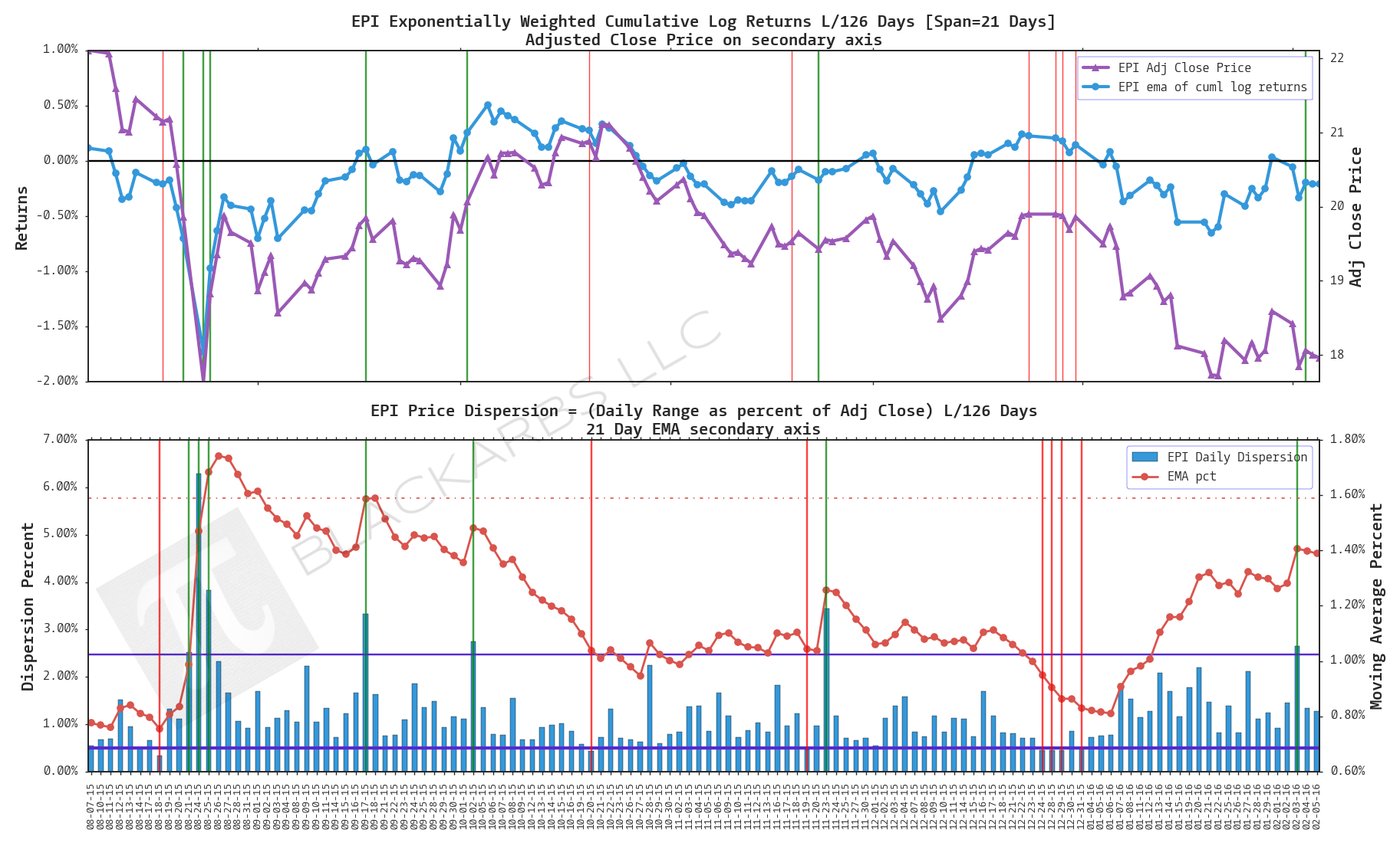
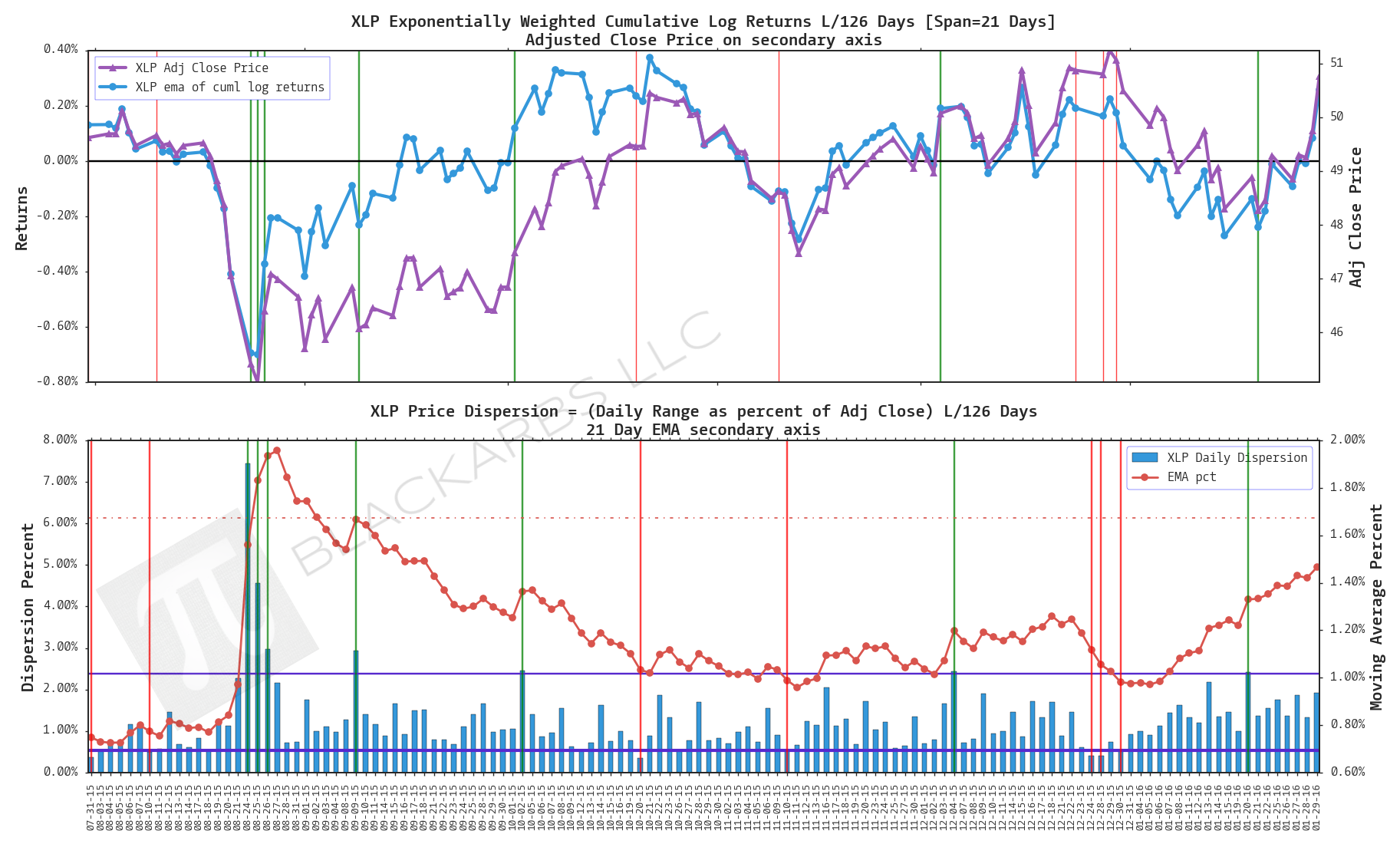
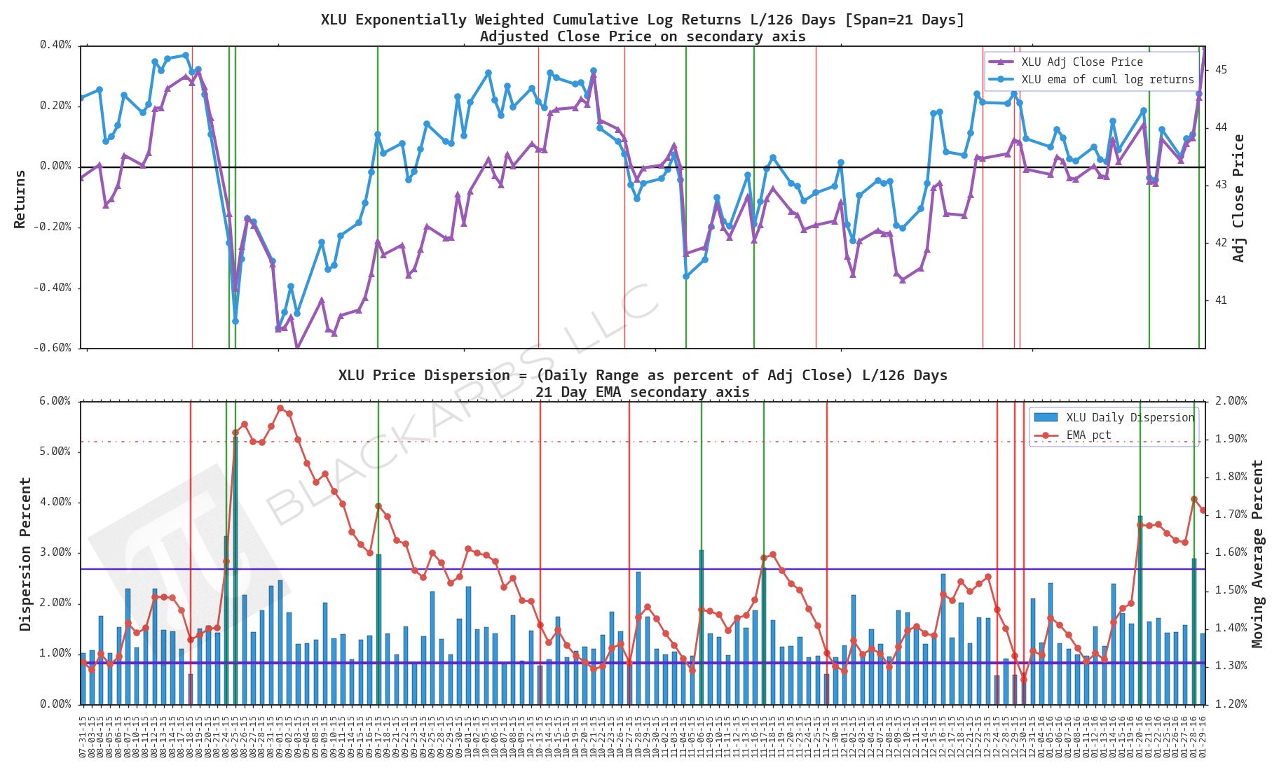
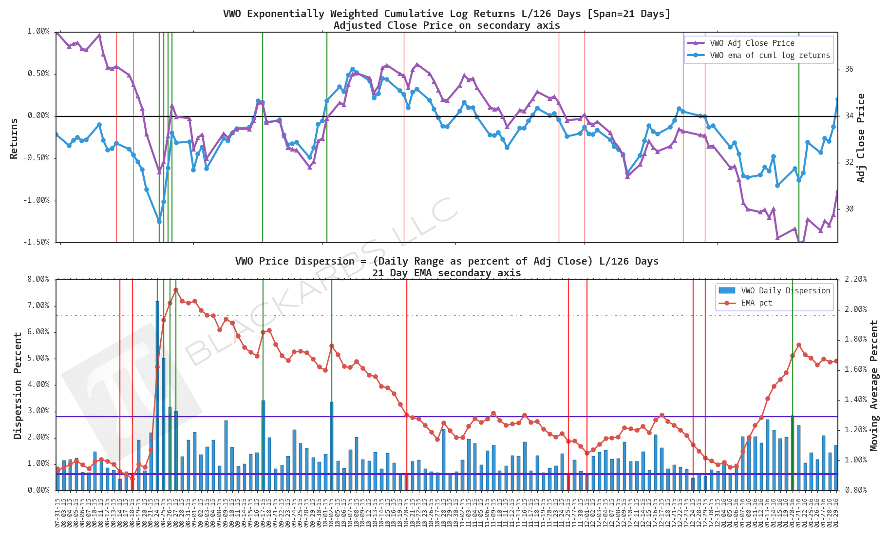
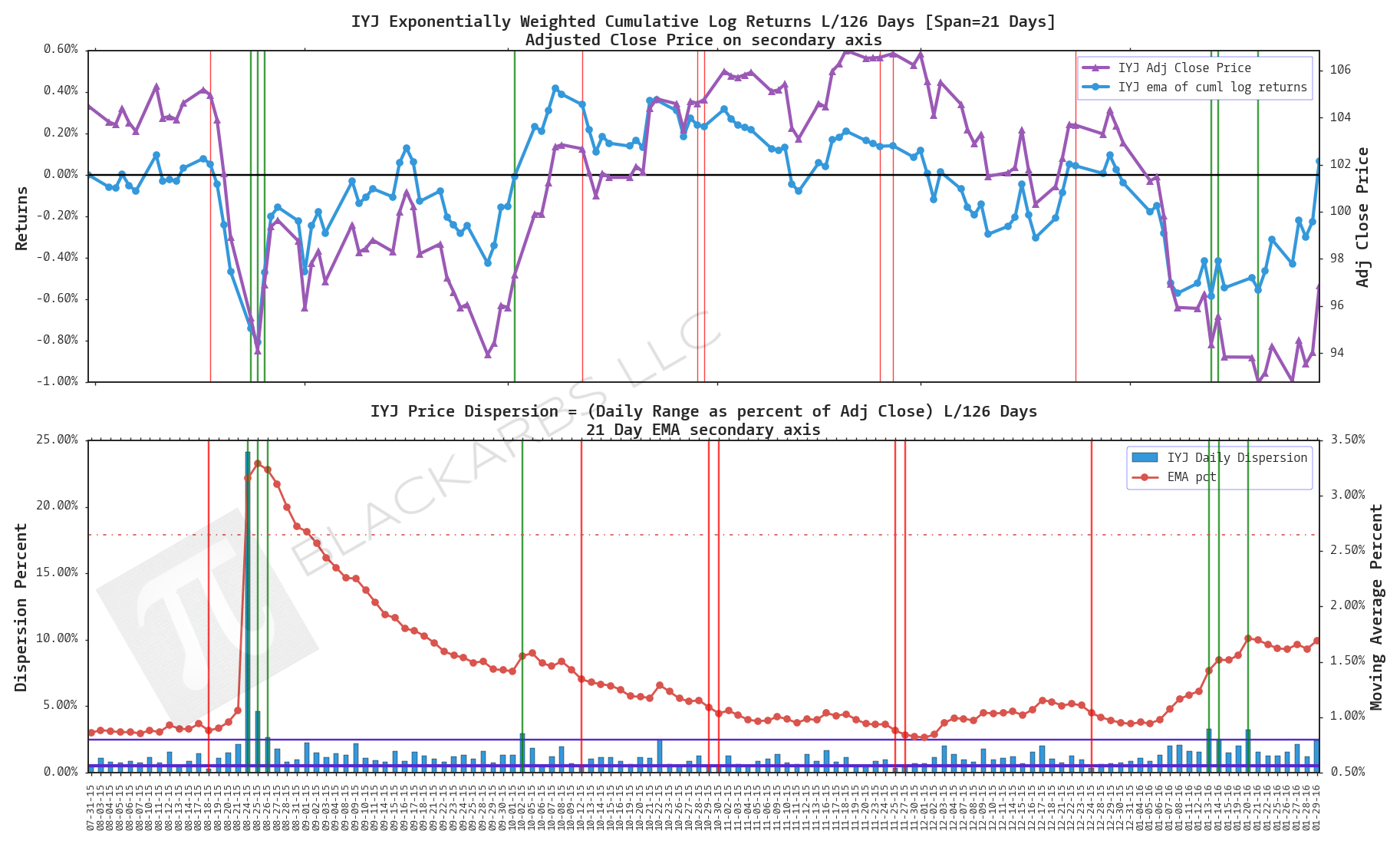
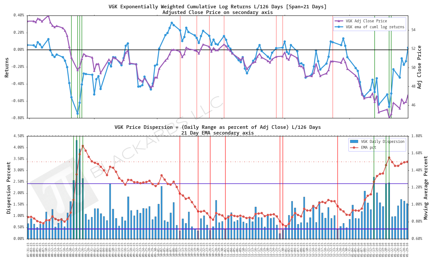
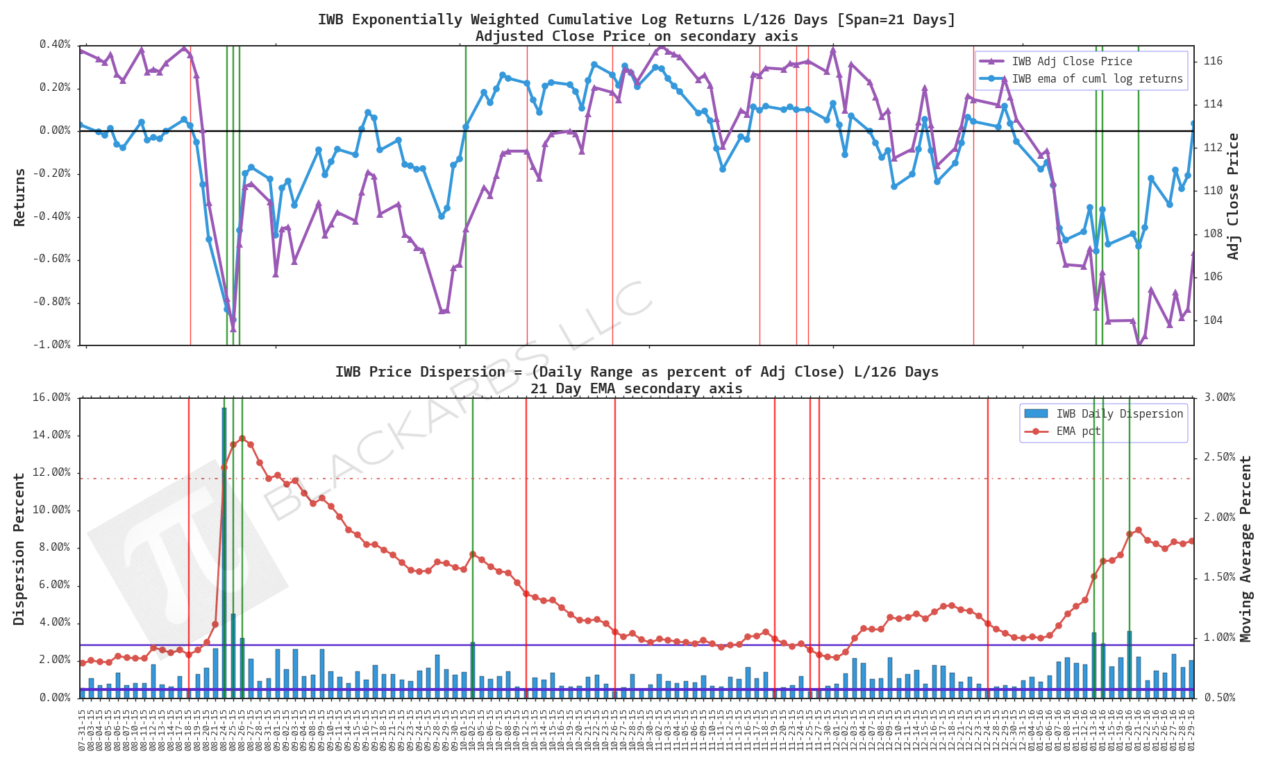
COMPOSITE ETF COMPONENTS:
LAST 252 TRADING DAYS


LAST 126 TRADING DAYS


LAST 63 TRADING DAYS


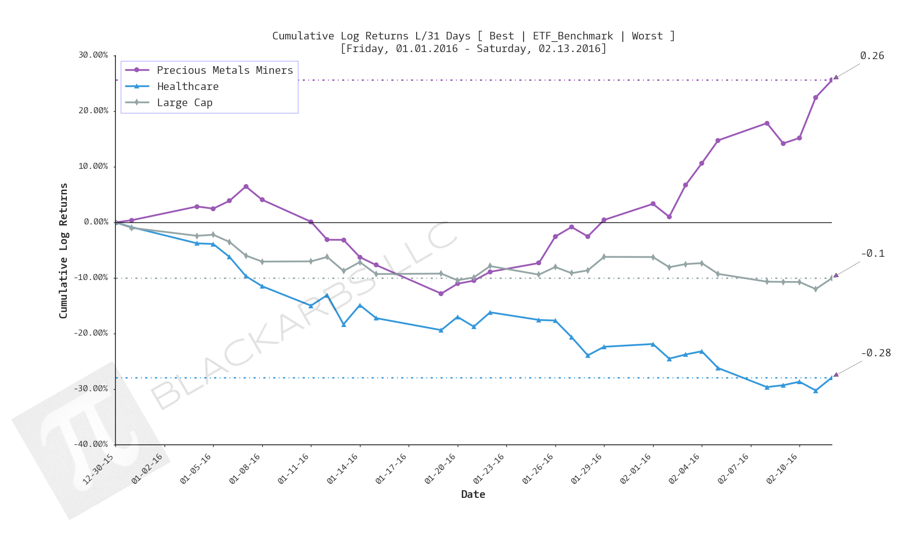
year-to-date LAST 31 TRADING DAYS


LAST 21 TRADING DAYS


LAST 10 TRADING DAYS


Implied Cost of Capital Estimates:
To learn more about the Implied Cost of Capital see here.
CATEGORY AVERAGE ICC ESTIMATES
ALL ETF ICC ESTIMATES BY CATEGORY
Cumulative Return Tables:
Notable Observations and Trends:
- Investors appear to be increasing their defensive positioning in the market as evidenced by the continued relative strength in the Precious Metals/Precious Metals Miners and Treasury Bond composites.
- Investors appear to be liquidating previous high performing asset classes as evidenced by Healthcare being among the bottom 3 performers off all composites across 5/6 timeframes beginning over the last 126 days.
- This is also supported by further deterioration in the relative performance of the Technology composite, which appears as a bottom 3 performer year-to-date.
- Correlations still appear relatively binary. However, a notable change is occurring in the correlation of Oil and Gas with the rest of the Sector based composites. It appears to be weakening year-to-date as compared to the last 126/252 trading days.
- The Treasury bond composite is seeing a notable increase in its negative correlation with the rest of the market as well. I look for this trend to continue as long as the global Negative-Interest Rate Policy trend continues. The US offers relatively high yield when compared to negative rates!